Download

1 / 66
660 likes | 778 Views
Data Structures( 数据结构 ) Course 2:Searching. index 下标 , 索引 , 指针 sentinel 哨兵 probability 概率 key 关键字 hash 散列 , 杂凑 collision 冲突 cluster 聚集 , 群集 synonym 同义语 , 同义词 probe 探测 load factor 装填因子. Vocabulary. sequential search 顺序查找 element 元素 order 次序 binary search 二分查找

E N D
index 下标,索引,指针 sentinel 哨兵 probability 概率 key 关键字 hash 散列,杂凑 collision 冲突 cluster 聚集,群集 synonym 同义语,同义词 probe 探测 load factor 装填因子 Vocabulary • sequential search 顺序查找 • element 元素 • order 次序 • binary search 二分查找 • target 目标 • algorithm 算法 • array 数组 • location 位置 • object 对象,目标 • parameter 参数
One of the most common and time-consuming operations in computer science. To find the location of a target among a list of objects. Searching
Main contents(in chapter 2) • List searching(including two basic search algorithms) • Sequential search(including three variations) • Binary search • Hashed list searching—the key through an algorithmic function determines the location of data • Collision resolution • To discuss the list search algorithms using an array structure
2-1 list searches (work with arrays) • The algorithm used to search a list depends to the structure of list • Sequential search(any array) • List no ordered • Small lists • Not searched often
Locating data in unordered list Location wanted (3) A[0] A[1] A[11] Target given (14)
0 Index 14 not equal 4 A[0] A[1] A[11] 4 21 36 14 62 91 8 22 7 81 77 10 Index 1 14 not equal 21 A[11] A[0] A[1] … 4 21 36 14 62 91 8 22 7 81 77 10 Index 3 14 equal 14 A[11] A[0] A[1] 4 21 36 14 62 91 8 22 7 81 77 10 Search Concept Target given:14 Location wanted:3
Sequential search algorithms • Needs to tell the calling algorithm two things • Did it Find the data it was looking for? • If it did, at what index are the target data found. • Requires four parameters • The list we are searching • An index to the last element in the list • The target • The address where the found element’s index location is to stored (Return Boolean)
Locate the target in an unordered list Pre list must contain at least one element last is index to last element in the list target contains the data to be located locn is address of index in calling algorithm Post if found—matching index stored in locn & found true If not found—last stored in locn & found false Returnfound<boolean> sequential search algorithm algorithm seqsearch(val list <array> val last <index> val target <keytype> ref locn <index>) looker=0 loop (looker < last and target not equal list [looker]) looker = looker + 1 end loop locn = looker if (target equal list [looker]) found = true else found = false end if return found end seqsearch
Variations on sequential searches • Sentinel search • Probability search • Ordered list search
Locate the target in an unordered list Pre list must contain at least one element Last is index to last element in the list Target contains the data to be located Locn is address of index in calling algorithm Post if found—matching index stored in locn & found true If not found—last stored in locn & found true Returnfound<boolean> Sentinel search algorithm seqsearch(val list <array> val last <index> val target <keytype> ref locn <index>) List [last + 1] = target looker=0 loop (target not equal list [looker]) looker = looker + 1 end loop locn = looker if (looker <= last) found = true locn = looker else found = false locn = last end if return found end sentinel search
probability search looker=0 loop (looker < last and target not equal list [looker]) looker = looker + 1 end loop if (target equal list [looker]) found = true if ( looker > 0 ) temp = list [looker – 1] list [looker – 1] = list [looker] list [looker] = temp looker = looker – 1 endif else found = false end if locn = looker return found end probability search Locate the target in an unordered list Pre as the same above Post if found—matching index stored in locn & found true & Element move up in priority If not found—as same Returnfound<boolean>
Locate target in a list ordered on target • Note: • It is not necessary to search to the end of list • It is only for the small list • Incorporate the Sentinel • Pre: the same as sequential • Post • if found—the same as above • If not found—locn is index of first element > target or locn equal last & found is false • Returnfound < boolean > Ordered list search If (target <= list[last ] ) looker=0 loop (target > list [looker]) looker = looker + 1 end loop else looker = last endif if (target equal list[looker]) found = true else found = false end if locn = looker return found
Binary search • Sequential search algorithm is very slow • But, It is the only solution if the array is not sorted • Binary search(ordered list) • For the large list • First sort • Then search
Binary search method • Suppose • L a sorted list • searching for a value X • Compare X to the middle value (M) in L. • if X = M we are done. • if X < M we continue our search, but we can confine our search to the first half of L and entirely ignore the second half of L. 4.if X > M we continue, but confine ourselves to the second half of L.
First mid last Target are found ,target 22 is in the list 0 5 11 A[0] A[1] A[11] 4 7 8 10 14 21 22 36 62 77 81 91 22>21 6 8 11 A[0] A[1] A[11] 4 7 8 10 14 21 22 36 62 77 81 91 22<62 First mid last 6 6 7 A[0] A[1] A[11] 4 7 8 10 14 21 22 36 62 77 81 91 22=22 First mid last
Target not found --Target 11 is not in the list First mid last 0 5 11 11<21 A[0] A[11] 4 7 8 10 14 21 22 36 62 77 81 91 First mid last 0 2 4 11>8 A[0] A[1] A[11] 4 7 8 10 14 21 22 36 62 77 81 91 First mid last 11>10 3 3 4 A[0] A[1] A[11] 4 7 8 10 14 21 22 36 62 77 81 91 First mid last 4 4 4 11<14 A[0] A[1] A[11] 4 7 8 10 14 21 22 36 62 77 81 91 First mid last Function terminates 4 4 3
Prelist is ordered; it must contain at least one element end is index to the largest element in the list Target is the value of element being sought Locn is address of index in calling algorithm Post Found:locn assigned index to target element found set true not found:locn = element below or above target found set false Returnfound<boolean> Binary search(ordered list) else found equal : force exit first = last + 1 end if end loop locn = mid if (target equal list [mid]) found = true else found = false end if return found end binary search algorithm binary_search( val list <array>, val end <index>, val target <keytype>, ref locn <index>) First = 0 Last = end loop (first <= last ) mid = ( first + last ) / 2 if ( target > list [mid] ) look in upper half first = mid +1 else if ( target < list [mid] ) look in lower half last = mid – 1
Analyzing (the efficiency) • Sequential search ,Sentinel search ,Ordered list search : O(n) • Binary search: O(log 2n) • Comparison of binary and sequential searches
Location of data key Hash function index of array(address of list ) key Hash algorithm 2-3 Hashed list searches Ideal search : we would know exactly where the data are and go directly to there Goal of hashed search : to find the data with only one test Use an array of data
[000] Harry lee [001] [002] 111060 Sarah trapp [003] [004] 102002 Vu nguyen [005] [006] [007] [008] … … [099] 107095 John adams [100] Hash function address key address 5 102002 107095 111060 100 hash 2 key Figure 2-6 Hash concept
Basic Concepts Hash search: A search in which the key ,through an algorithmic function, determines the location of the data. we use a hashing algorithm to transform the key into the index that contains the data we need to locate (key-to –address)
Problem A set of keys hash to the same location—Synonym Contain two or more synonyms in a list—collision Home address—produced by hashing algorithm Prime area—memory contains all of home addresses Collision resolution—two keys collide at a home address Place one of the keys and its data in another location
B and A Collide at 8 Collision resolution C and B Collide at 16 [0] [4] [16] [8] Collision resolution 1.hash(A) 3.hash(C) 2.hash(B) Figure 2-7 the collision resolution concept
Locate an element in a hashed list Use the same algorithm to insert it into the list First hash the key and check the home address If it does – the search is complete If not – use the collision resolution algorithm to determine the next location and continue until find the element or determine it is not in the list Each calculation of an address and test for success – probe
Hashing methods Hashing methods direct modulo division midsquare rotation pseudorandom generation digit extraction subtraction folding Figure 2-8 Basic hashing techniques
Direct method • The key is the address(an element a key , no synonyms) • Example1: total monthly sales by the days of the months • Create an array of 31accumulator • The accumulation code is: dailySales[sale.day] = dailySales[sale.day] +sale.amount;
Example 2: a small company has fewer<100 Employee number is between 1 and 100 [000] [001] [002] [003] address [004] 5 [005] 005 100 002 100 hash [006] 2 [007] [008] key Figure 2-9 Direct hashing Of employee numbers [099] [100]
Subtraction method • keys are consecutive , but do not start from 1 • Such as your student ID number • Advantage • Hashing function is very simple • No collisions • Disadvantage • Only for small lists
Note: 1. Generally speaking , hashing lists require some empty elements to reduce the number of collisions 2. This application above two is the ideal ,but it is very limited , such as ID card number
Modulo-division method(Division remainder) This method divides the key by the array size and uses the remainder for the address Hashing algorithm is: Address = key modulus listsize Note: a prime number listsize produces fewer collisions
[000] [001] [002] 2 [003] 121267 045128 379452 306 hash [004] 0 [005] [006] [007] [008] Listsize=307 [305] Figure 2-10 modulo-division Hashing [306]
Digit extraction method Selected digits are extracted from the key And used as address Example 379452 121267 378845 160252 045128 394 112 388 102 051 6-digits Employee number 3-digit address Select the first, third, fourth digits
Midsquare method The key is squared and the address selected from the middle of the squared number Limitation: the size of the key Example: 4-digit keys 9452*9452=89340304:address is 3403 Variation : select a portion of the key 379452 121267 378845 160252 045128 379 * 379=143641 121 * 121=014641 378 * 378=142884 160 * 160=025600 045 * 045=002025 364 464 288 560 202 Select 3-5 digits as address Select 1-3 digits squared Fill 0 to 6 digits
Folding methods : fold shift and fold boundary 123456789 Digits reversed 321 123 123 456 789 123 456 789 + + 987 789 Digits reversed 764 1 1 368 discarded discarded (b)fold boundary (a)fold shift Figure 2-11 hash fold examples
Rotation method : Incorporate with others Useful when keys are assigned serially 600101 600102 600103 600104 600105 600101 600102 600103 600104 600105 160010 260010 360010 460010 560010 Original key Rotation Rotated key Figure 2-12 Rotation hashing
Pseudorandom method: In this method, the key is used as the seed in a pseudorandom number generator , the resulting random number is scaled into the possible address range using modulo division A common random generator is: y=ax+c For efficiency,factors a and c should be prime numbers For example , a=17, c=7
(17*045128+7) modulo 307=297 [000] (17*121267+7) modulo 307=41 [007] 41 121267 045128 379452 [041] 297 hash 7 (17*379452+7) modulo 307=7 [297] Figure 2-10 modulo-division Hashing [306]
Hash Algorithm • Convert the alphanumeric key into a number by adding the American Standard Code for Information Interchange(ASCII) to accumulator. • Rotate the bits in the address to maximize the distribution of the values. • Take the absolutely value of the address and map it into the address range.
This algorithm converts an alphanumeric key of size characters into an integral address. Pre Key is a key to be hashed. size is the number of characters in the key. MaxAddr is the maximum possible address for the list. Post addr contain the hashed address Hash Algorithm algorithm Hash( val key <array >, val size <integer>, val maxAddr <integer>, ref addr <integer>) Looper = 0 Addr = 0 Hash Key Loop (Loop<size) if (key[looper] not space) addr =addr+key[looper] rotate addr 12 bits right end if End loop test for negative address if (addr<0) addr=absolute(addr) end if addr =addr modulo maxaddr return end Hash
2-4 collision resolution • Except the direct and subtraction, none of the hashing methods are one-to-one mapping • Collision not avoid • There are several methods for hashing collisions Collision resolution Open addressing Linked lists buckets pseudorandom Key offset Linear probe Quadratic probe Figure 2-13 collision resolution methods
Several concepts • data to group within the list (unevenly across a hashed list). • a high degree of clustering grows the number of probes to locate an element and reduces the processing efficiency of the list. There are two: • Primary clustering : when data cluster around a home address • Secondary clustering:when data become grouped along a collision path throughout a list • Need to design hashing algorithms to minimize clustering • load factor • Clustering • There must be some empty elements in a list: The number of filled elements load factor <75% = The total number of elements
Open addressing • Resolves collisions in the prime area (contains all of the home addresses ) • Linear probe • Quadratic probe • Double hashing • Pseudorandom • Key offset
Linear Probe [000] [001] [002] First insert: No collision [003] [004] 1 070918 166702 [005] hash [006] 1 [007] [008] second insert: collision Add 1 [305] Figure 2-14 linear probe collision resolution [306]
linear probe Variation :Add 1, subtract 2,Add 3, subtract 4 Advantage: simple to implement. Disadvantage: first, tend to produce primary clustering . Second, tend to make the search algorithm more complex
Quadratic probe • To eliminate primary clustering • The increment is the collision probe number squared.first probe, add 12,second probe, add 22 ,… • The new address is the modulo of the list size. • Disadvantage : 1. the time required to square the probe number. 2. It is not possible to generate a new address for every element in the list.
Pseudorandom collision resolution • A double hashing : the address is rehashed • Uses a pseudorandom number to resolve the collision • Using the collision address as a factor in the random number calculation, such as: New address = 3 * collision address + 5 Figure2-15 showing a collision resolving for figure 2-14
Pseudorandom probe [000] [001] [002] First insert: No collision [003] [004] 1 [005] 070918 166702 hash [006] 1 [007] [008] second insert: collision Pseudorandom Y = 3x+5 [305] [306] Figure 2-15 pseudorandom collision resolution
Key offset • Another double hashing • Produces different collision paths for different keys • key offset calculates the new address as (the simplest versions) offset = key/listsize address = ((offset + old address) modulo listsize)