Download
1 / 32
320 likes | 480 Views
Integration of Design and Control: A Robust Control Approach. by Nongluk Chawankul Peter L. Douglas Hector M. Budman University of Waterloo Waterloo, Ontario, Canada. Background. Control performance depends on the controller and the design of the process.

E N D
Integration of Design and Control: A Robust Control Approach by Nongluk Chawankul Peter L. Douglas Hector M. Budman University of Waterloo Waterloo, Ontario, Canada
Background • Control performance depends on the controller and the design of the process. Traditional design procedure: • Step 1: Process design (sizing + nominal operating conditions) • Step 2: Control design • Idea of integrating design and control: Integrated approach Process design Process control + =
Background Traditional design and control design Integrated design and control design Only one step design Two steps design Step 1: Process design Objective Function (Cost) Cost = Capital cost(x) + operating cost(x) where x is design variable Cost = capital cost(x) + operating cost(x) + cost related to closed loop system(x,y) where x is design variable y is control tuning parameter Min Cost(x) x s.t. h(x) = 0 g(x) 0 Optimum design • Process constraints • Equality constraints, h(x) = 0 • Inequality constraints, g(x,y) 0 Step 2: Control design Min Cost(x,y) x,y s.t. h(x) = 0 g(x,y) 0 Design controller Closed loop system Optimum design
Integrated Design and Control Design Previous studies Our study • Linear Nominal Model + Model Uncertainty (Simple optimization problem) • Variability cost into cost function : One objective function • extended to Centralized Control : MPC • Nonlinear Dynamic Model (difficult optimization problem) • Variability cost not into cost function: Multi-objective optimization • Decentralized Control : PI /PID
Case study • Case study II: SISO MPC • Case study III: MIMO MPC SISO system MIMO system XD XD RR RR A A1 + + - XD* Feed Feed IMC or MPC - XD* MPC Ethane Propane Isobutane N-Butane N-Pentane N-Hexane Ethane Propane Isobutane N-Butane N-Pentane N-Hexane Q - XB* Q + A2 XB XB
Case Study III: MIMO MPC MIMO case study: • RadFrac model in ASPEN PLUS was used. • Different column designs, 19 – 59 stages were studied. • Product specifications • Mole fraction of propane in distillate product = 0.783 • Mole fraction of isobutane in bottom product = 0.1 • Design variables are functions of nominal RR at specific product compositions.
Optimization Minimize Cost(U,C) = CC(U) + OC(U) + max VC(U,C) U,CLm Such that h(U) = 0 (equality constraints) g(U,C) 0 (inequality constraints) Objective Function U is a vector of design variables. C is a vector of control variables. Lm is a set of uncertainty.
Capital Cost (CC) and Operating Cost (OC) • Capital Cost, CC • Cost of sizing, e.g. number of stages N and column diameter D • Capital cost for distillation column from Luyben and Floudas, 1994 ($/day) • Operating Cost, OC • Operating cost from Luyben and Floudas, 1994 ($/day) where tax = tax factor HD = reboiler duty (GJ/hr) OP = operating period (hrs) UC = Utility cost ($/GJ)
Variability Cost (VC) Variability Cost, VC - Variability cost, VC = inventory cost • sinusoid disturbance induces process variability • consider holding tank to attenuate the product variation t V1 t RR A1 + - XD* Feed t MPC Ethane Propane Isobutane N-Butane N-Pentane N-Hexane Q - XB* + A2 V2 t t
Calculation of Variability Cost (VC) - 1 Assume, W is sinusoidal disturbance with specific d. (alternatively, superposition of sinusoids) With phase lag Consider worst case variability : Related to maximum VC
Calculation of Variability Cost (VC) - 2 Objective Function (-cont-) Cin Cout V Q in Q out Apply Laplace transform The product volume in the holding tank VC1 = W1P1V1(A/P,i,N) VC2 = W2P2V2(A/P,i,N) VC = VC1+ VC2
Equality Constraints: Process models -1 Process Models: ASPEN PLUS simulations at specific product compositions Q(RR) N(RR) D(RR) HD(RR)
Equality Constraints: Process models - 2 Process Models: ASPEN PLUS simulations BF(RR) DF(RR)
y -35% 35% +35% y1 -1% 1% y2 +1% time 0 Process Models: Input/Output Model for 22 system Equality Constraints: Process models - 3 yi Sn S3 • First Order Model S2 S1 t Process gains and • Kp1(RR) for paring xD-RR • Kp2(RR) for paring xB-RR • Kp3(Q) for paring xD-Q • Kp4(Q) for paring xB-Q • In a similar fashion, time constants and dead time • p(RR) and p(Q) • (RR)
Equality Constraints: Process models - 4 Process gains for 2 2 system
Equality Constraints: Process models - 5 Process time constants: p(RR) and p(Q) Process dead time: (RR)
y Time Equality Constraints: Process models - 6 • Model uncertainty Sn,upper Sn,nom xD-RR Sn,lower xB-RR xD-Q xB-Q
Equality Constraints: Process models - 7 Model Uncertainty for 22 system
Inequality Constraints- 1 is a tuning parameter. Large less aggressive control Manipulated variable constraint Two manipulated variables Calculate RR and Q and
Inequality Constraints- 2 Block diagram of the MPC and the connection matrix M M Z(k) w(k) U(k) W1 W2 Z-1I (k+1/k) u(k) U(k-1) + T2 N1 + Li Kmpc T1 + + H + - 2. Robust stability constraint (Zanovello and Budman, 1999) H N1 + + Mp H - + N2 Z-1I U(k+1) U(k) M z w
Two different approaches Traditional Method • Integrated Method Robust Performance (Morari, 1989) Where U is manipulated variables
Results - 1 Results from Integrated design and control design approach • w1 or w2 increases; • RR* decreases smaller dead time • 11 decreases interaction decreases as RR decreases • * decreases RS constraint is easy to satisfy as 11 decreases
Results - 2 Compare Results from Traditional and Integrated design and control design approaches.
Results - 3 Effect of RRmax on Total Cost (TC)
Conclusions 1- For the case ≠ 0, using the integrated method, the optimization tends to select smaller RR values which correspond to smaller dead time and smaller interaction. 2- The optimal design obtained using the integrated method resulted in a lower total cost as compared to the traditional method. 3- Limit on manipulated variable affects the closed loop performance and leads to more cost.
Calculation of Variability Cost (VC) -1 Process variability W (Sinusoid unmeasured disturbance) r=0 y u + MPC Process + + - Substitute (k), u(k-1) into the first equation and apply z-transform
Results - 1 Results from Integrated design and control design approach for = 0 • w1 or w2 increases; • RR* increases uncertainty decreases as RR increases • 11 increases interaction increases as RR increases • * increases RS constraint is more difficult to satisfy as 11 increases
Results - 4 Compare savings when = 0 and 0 = 0 0 = 0 0