Download
1 / 89
900 likes | 989 Views
Phase: An Important Low-Level Image Invariant Peter Kovesi School of Computer Science & Software Engineering The University of Western Australia. Canny. Canny. Much of computer vision depends on the ability to correctly detect, localize and match local features.

E N D
Phase: An Important Low-Level Image Invariant Peter Kovesi School of Computer Science & Software Engineering The University of Western Australia
Much of computer vision depends on the ability to correctly detect, localize and match local features
Much of computer vision depends on the ability to correctly detect, localize and match local features • But… • Edges, corners and other features are not simple step changes in luminance.
Much of computer vision depends on the ability to correctly detect, localize and match local features • But… • Edges, corners and other features are not simple step changes in luminance. • Gradient based operators do not correctly detect and localize many image features.
Much of computer vision depends on the ability to correctly detect, localize and match local features • But… • Edges, corners and other features are not simple step changes in luminance. • Gradient based operators do not correctly detect and localize many image features. • The localization of gradient based features varies with scale of analysis.
Much of computer vision depends on the ability to correctly detect, localize and match local features • But… • Edges, corners and other features are not simple step changes in luminance. • Gradient based operators do not correctly detect and localize many image features. • The localization of gradient based features varies with scale of analysis. • Thresholds are sensitive to image illumination and contrast.
Much of computer vision depends on the ability to correctly detect, localize and match local features • But… • Edges, corners and other features are not simple step changes in luminance. • Gradient based operators do not correctly detect and localize many image features. • The localization of gradient based features varies with scale of analysis. • Thresholds are sensitive to image illumination and contrast. • Despite the obvious importance of edges we do not really know how to use them.
Corners Advances in reconstruction algorithms have renewed our interest in, and reliance on, the detection of feature points or ‘corners’. Pollefeys’ castle
What’s the Problem? • Current corner detectors do not work reliably with images of varying lighting and contrast. • Localization of features can be inaccurate and depends on the scale of analysis.
Harris Operator Form the gradient covariance matrix where and are image gradients in x and y A corner occurs when eigenvalues are similar and large. Corner strength is given by (k = 0.04) Note that R has units (intensity gradient)4
The Harris operator is very sensitive to local contrast Test image Fourth root of Harris corner strength (Max value is ~1.5x10¹⁰)
The location of Harris corners is sensitive to scale Harris corners, s = 1 Harris corners, s = 7
Gradient based operators are sensitive to illumination variations and do not localize accurately or consistently. As a consequence, successful 3D reconstruction from matched corner points requires extensive outlier removal and the application of robust estimation techniques.
Gradient based operators are sensitive to illumination variations and do not localize accurately or consistently. As a consequence, successful 3D reconstruction from matched corner points requires extensive outlier removal and the application of robust estimation techniques. To minimize these problems we need a feature operator that is maximally invariant to illumination and scale.
Features are Perceived at Points of Phase Congruency • Do not think of features in terms of derivatives! • Think of features in terms of local frequency components. • The Fourier components are all in phase at the point of the step in the square wave, and at the peaks and troughs of the triangular wave. • Features are perceived where there is structure in the local phase. (Morrone & Owens 1987)
+ = Phase and amplitude mixed image (Oppenheim and Lim 1981)
phase offset amplitude decay with frequency Phase Congruency Models a Wide Range of Feature Types A continuum of feature types from step to line can be obtained by varying the phase offset. Sharpness is controlled by amplitude decay.
Congruency of Phase at any Angle Produces a Feature Interpolation of a step to a line by varying from 0 at the top to at the bottom
Measuring Phase Congruency x Phase Congruency is the ratio Polar diagram of local Fourier components at a location x plotted head to tail: Amplitude Phase Local Energy
Failure of a gradient operator on a simple synthetic image… Section A-A Section B-B A gradient based operator merely marks points of maximum gradient. Note the doubled response around the sphere and the confused torus boundary. Canny edge map
Phase Congruency edge map Feature classifications Test grating Feature classifications
log frequency Implementation Calculate local frequency information by convolving the image with banks of quadrature pairs of log-Gabor wavelets (Field 1987). even-symmetric wavelets (real-valued) odd-symmetric wavelets (imaginary-valued) amplitude
For each point in the signal the responses from the quadrature pairs of filters at different scales will form response vectors that encode phase and amplitude.
Implementation Local frequency information is obtained by applying quadrature pairs of log-Gabor filters over six orientations and 3-4 scales (typically). sine Gabor cosine Gabor
Implementation Local frequency information is obtained by applying quadrature pairs of log-Gabor filters over six orientations and 3-4 scales (typically). Phase Congruency values are calculated for every orientation - how do we combine this information?
Detecting Corners and Edges At each point in the image compute the Phase Congruency covariance matrix. where PCx and PCy are the x and y components of Phase Congruency for each orientation. The minimum and maximum singular values correspond to the minimum and maximum moments of Phase Congruency.
M m • The magnitude of the maximum moment, M, gives an indication of the significance of the feature. • If the minimum moment, m, is also large we have an indication that the feature has a strong 2D component and can be classified as a corner. • The principal axis, about which the moment is minimized, provides information about the orientation of the feature.
Comparison with Harris Operator • The minimum and maximum values of the Phase Congruency singular values/moments are bounded to the range 0-1 and are dimensionless. This provides invariance to illumination and contrast. • Phase Congruency moment values can be used directly to determine feature significance. Typically a threshold of 0.3 - 0.4 can be used. • Eigenvalues/Singular values of a gradient covariance matrix are unbounded and have units (gradient)4 - the cause of the difficulties with the Harris operator.
Edge strength - given by magnitude of maximum Phase Congruency moment. Corner strength - given by magnitude of minimum Phase Congruency moment.
Fourth root of Harris corner strength (max value ~1.25x10¹⁰) Image with strong shadows
Phase Congruency edge strength (max possible value = 1.0) Phase Congruency corner strength (max possible value = 1.0)
Harris corners thresholded at 108 (max corner strength ~1.25x10¹⁰) Phase Congruency corners thresholded at 0.4
Good Things: • Phase Congruency is a dimensionless quantity. • Invariant to contrast and scale. • Value ranges between 0 and 1. • 0 1 • no congruency perfect congruency • Threshold values can be fixed for wide classes of images. • Provides classification of features.
Problems: • Degenerates when Fourier components are very small. • Degenerates when there is only one Fourier component. • Sensitive to noise. • Localization is not sharp.
A Degeneracy with a single frequency component • Congruency of phase is only significant if it occurs over a distribution of frequencies. • What is a good distribution? • Natural images have an amplitude spectrum that decay at • (Field 1987) weighting function for frequency spread small constant to avoid division by 0
Noise • Being a normalized quantity Phase Congruency is sensitive to noise. • The radius of the noise circle represents the value of |E(x)| one can expect from noise. • If E(x) falls within this circle our confidence in any Phase Congruency value • falls to 0.
Noise Compensation Calculate Phase Congruency using the amount that |E(x) | exceeds the radius of the noise circle, T.
Radius of the Noise Circle… The radius of the noise circle is the expected distance from the origin if we take an n-step random walk in the plane • The size of the steps correspond to the expected noise response • of the filters at each scale. • The direction of the steps are random.
noise spectrum Radius of the Noise Circle… If we assume the noise spectrum is flat filters will gather energy from the noise as a function of their bandwidth (which is proportional to centre frequency). Smallest wavelet has largest bandwidth gets the most energy from noise. Smallest wavelet has the most local response to features in the signal most of the time it is only responding to noise.
Gaussian white noise Convolve with even & odd smallest scale wavelets odd response filter response vectors even response The distribution of the positions of the response vectors will be a 2D Gaussian ( + some contamination from feature responses). We are interested in the distribution of the magnitude of the responses - This will be a Rayleigh Distribution. Mean Variance are described by one parameter
To obtain a robust estimate of for the smallest scale filter we find the median response of the filter over the whole image. This minimizes the influence of any contamination to the distribution from responses to features. • and the median have a fixed relationship. • Get median get get • Expected noise responses at other scales are determined by the bandwidths of the other filters relative to the smallest scale filter pair. • Given the expected filter responses we can solve for the expected distribution of the sum of the responses (which will be another Rayleigh distribution). Set noise threshold in terms of the overall distribution. 2 - 3