Bayesian Networks

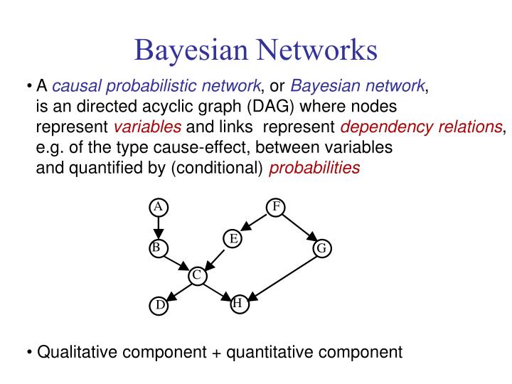
Bayesian Networks • A causal probabilistic network, or Bayesian network, • is an directed acyclic graph (DAG) where nodes • represent variables and links represent dependencyrelations, • e.g. of the type cause-effect, between variables • and quantified by (conditional) probabilities • Qualitative component + quantitative component

Bayesian Networks • Qualitative component : relations of conditional dependence / independence • I(A, B | C): A and B are independent given C • I(A, B) = I(A, B | Ø): A and B are a priori independent • Formal study of the properties of the ternary relation I • A Bayesian network may encode three fundamental types • of relations among neighbour variables.

Qualitative Relations : type I FGH Ex: F: smoke, G: bronchitis, H: respiratory problems (dyspnea) Relations: ¬ I(F, H) I(F, H | G)

Qualitative Relations : type II EFG Ex: F: smoke, G: bronchitis, E: lung cancer Relations: ¬ I(E, G) I(E, G | F)

Qualitative Relations : type III B  C  E Ex: C: alarm, B: movement detection, E: rain Relations: I(B, E) ¬ I(B, E | C)

Probabilistic component • Qualitative knowledge: a directed acyclic graph G (DAG) Nodes(G) = V = {X1, …, Xn} -- discrete variables -- Edges(G)  VxV Parents(Xi) = {Xi : (Xj, Xi)  Edges(G)} • Probabilistic knowledge: P(Xi | parents(Xi)) • These probabilities determine a joint probability distributionP over V = {X1, …, Xn}: • P(X1, …, Xn) = P(X1 | parents(X1)) · · · P(Xn | parents(Xn)) • Bayesian Network = (G, P)

Joint Distribution • P(X1,X2,...Xn) = P(Xn|Xn-1,...X1) ... P(X3|X2,X1) P(X2|X1) P(X1). • Independence relations of each variable Xi with the set of predecessor variables of the parents of Xi: • P(Xi | parents(Xi), Y1,.., Yk) = P(Xi | parents(Xi)) • P(X1, X2, ..., Xn) = i=1,n P(Xi | parents(Xi)) • • to have in each node Xi the conditional probability distribution P(Xi | parents(Xi)) is enough to determine the full joint probability distribution P(X1,X2,...,Xn)

Example A: visit to Asia B: tuberculosis F: smoke E: lung cancer G: bronchitis C: B or E D: X-ray H: dyspnea P(A): P(a) = 0.01 P(B | A): P(b | a) = 0.05, P(b | ¬a) = 0.01 P(C | B,E): P(c | b, e) = 1, P(c | b, ¬e) = 1, P(c | ¬b, e) = 1, P(c | ¬b, ¬e) = 0 P(F): P(f) = 0.5 P(D | C): P(d | c) = .98, P(d | ¬c) = 0.05 P(E | F): P(e | f) = 0.1, P(e | ¬f) = 0.01 P(G | F): P(g | f) = 0.6, P(g | ¬f) = 0.3 P(H | C, G): P(h | c,g) =0.9 , P(h | c,¬g) = 0.7, P(h | ¬c,g) = 0.8, P(h | ¬c,¬g) = 0.1, P(A,B,C,D,E,F,G,H) = P(D | C) P(H | C, G) P(C | B, E) P(G | F) P(E | F) P(F) P(B | A) P(A) P(a,¬b,c,¬d,e,f,g,¬h) = P(¬d |c) P(¬h |c,g) P(c | ¬b,e) P(g | f) P(e | f) P(f) P(¬b | a) P(a) = (1- 0.98)  (1-0.9)  1  0.6  0.1  0.5  (1-0.05)  0.01 = 5,7  10-7.

D-separation relations and probabilistic independence • Goal: precesely determine which independence relations (graphically) are defined by one DAG. • Previous definitions: • A path is a sequence of connected nodes in the graph. • A non directedpath is a path without taking into account the directions of the arrows. • A “head-to-head” link in a node is a (non directed) path of the form xyw, the node y is clalled a “head-to-head” node.

D-separation • • A path c is called to be activated by a set of nodes Z if the following two conditions are satisfied: • Every node in c with links head-to-head is in Z or it has a descendent in Z. • Any other node in c does not belong to Z. • Otherwise, the path c is called to be blockedby Z. • Definition. If X, Y and Z are three disjoint subsets of nodes disjunts in a DAG G, then Z d-separates X from Y, or equivalently X and Y are graphically independent given Z, when all the paths between any node from X and any node from Y are blocked by Z

D-separation {B} and {C} are d-separated by {A}: Path B-E-C: E,G  {A} - {A} blocks the path B-E-C Path B-A-C: - {A} blocks the path B-A-C Theorem. Let G be a DAG and let X,Y and Z be subsets of nodes such that X and Y are d-separated by Z. Then, X and Y are conditionally independent from Z for any probability P such that (G, P) is a causal network over G, that is, s.t. P(X | Y,Z) = P(X | Z) and P(Y | X,Z) = P(Y | Z).

Inference in Bayesian Networks Knowledge about a domain encoded by a Bayesian network XB = (G, P). Inference = updating probabilities: evidence E on values taken by some variables modify the probabilities of the rest of variables P(X) --- > P’(X) = P(X | E) Direct Method: XB = < G = {A,B,C,D,E}, P(A,B,C,D,E) > Evidence: A = ai, B = bj P(C = ck | A = ai, B = bj) =

Inference in Bayesian Networks • Bayesian networks allow local computations, which exploit the indepence relations among variables explictly induced by the corresponding DAG of the networks. • They allow updating the probability of a variable using only the probabilities of the immediat predecessor nodes (parents), and in this way, step by step to update the probabilities of all non-instantiated variables in the network ---> propagation methods • Two main propagation methods: • Pearl method: message passing over the DAG • Lauritzen & Spiegelhalter method: previous transformation of the DAG in a tree of cliques

Propagation method in trees of cliques transformation of initial network in another graphical structure, a tree of cliques (subsets de nodes)equivalent probabilistic information BN = (G, P)----> [Tree, P] propagation algorithm over the new structure

Graphical Transformation Definition: a “clique” in a non-directed graph is a complete and maximal subgraph To transform a DAG G in a tree of cliques: Delete directions in edges of G: G’ Moralization of G’: add edges between nodes with common sons in the original DAG G: G’’ Triangularization of G’’ : G* Identification of the cliques in G* Suitable enumeration of the cliques (Running Inters. Prop.) Construction of the tree according to the enumeration

Example(1) 1) 2)

Example (2): triangularization 3) 3)

Example (3): cliques Cliques: 4) Cliques: {A,B}, {B,C,E}, {E,F,G}, {C,E,G}, {C,G,H}, {C,D}

Ordering of cliques • Enumeration of cliques Clq1, Clq2, …, Clqn such that the following property holds: • Running Intersection Property: for all i=1,…, n there exists j < i such that SiClqj, where Si = Clqi(Clq1Clq2...Clqi-1). • This property is guaranteed if: • (i) nodes of the graph are enumerated following the criterion of “maximum cardinality search” • (ii) cliques are ordered according to the node of the clique with a highest ranking in the former enumaration.

Example (4): ordering cliques 1 6 3 2 5 4 8 7 Clq1 = {A,B}, Clq2 = {B,E,C}, Clq3 = {E,C,G}, Clq4 = {E,G,F}, Clq5 = {C,G,H}, Clq6 = {C,D}

Tree Construction Let [Clq1, Clq2, …, Clqn ] be an ordering satisfying R.I.P. For each clique Clqi, define Si = Clqi(Clq1Clq2...Clqi-1) Ri = Clqi-Si. Tree of cliques: - (hyper) nodes: cliques - root: Clq1 - for each clique Clqi, its “father” candidates are cliques Clqk with k < i and s.t. Si  Clqk (if more than one candidate, random selection)

Example (5): trees S2 = Clq2 Clq1{Clq1 S3 = Clq3(Clq1Clq2){E,CClq2 S4 = Clq4(Clq1Clq2 Clq3){GClq3 S5 = Clq5(Clq1Clq2 Clq3.Clq4){C,GClq3 S6 = Clq6( Clq1Clq2 Clq3.Clq4Clq5){CClq2, Clq3, Clq5

Propagation Algorithm • Potential Representationof the distribution P(X1, …, Xn): • ([W1...Wp], ) is a potential representation of P, where the Wi • are subsets of V = {X1, …, Xn}, if P(V) = • In a Bayesian network (G, P): • P(X1, ..., Xn) = P(Xn| parents(Xn))·...· P(X1| parents(X1)) • admits a potential representationP(X1, ..., Xn) = (Clq1) ·(Clq2) · ... · (Clqm) • with (Clqi)= ∏{P(Xj | parents(Xj)) | XjClqi, parents(Xj) Clqi ,

Propagation Algorithm (2) • Fundamental property of the potential representations: • Let ([W1, ..., Wm], ) be a potential representation for P. Evidence: X3 = a and X5 = b. • Problem: update the probabilitaty P’(X1, ..., Xn) = P(X1, ..., Xn| X3=a,X5 = b) ?? • Define: W^i = Wi - {X3, X5} ^(W^i) =  (Wi (X3=a, X5=b)) • ([W^1, ..., W^m], ^) is a potential representation for P'.

Example (6): potentials Clq1 = {A,B}, Clq2 = {B,E,C}, Clq3 = {E,C,G}, Clq4 = {E,G,F}, Clq5 = {C,G,H}, Clq6 = {C,D} P(A,B,C,D,E,F,G,H) = P(D | C) P(H | C, G) P(C | B, E) P(G | F) P(E | F) P(F) P(B | A) P(A) (Clq1) = P(A)· P(B | A) (Clq2) = P(C | B,E), (Clq3) = 1 (Clq4) = P(F).P(E | F).P(G | F), (Clq5) = P(H | C, G) (Clq6) = P(D | C) P(A,B,C,D,E,F,G,H) =(Clq1) • …. • (Clq6)

Propagation algorithm: theoretical resultats • Causal network (G, P)([Clq1, ..., Clqp], ) is a potential representation for P • 1) P(Clqi) = P(Ri|Si).P(Si) • 2) P(Rp|Sp) = , where is the marginal of the function  with respect to the variables of Rp. • 3) If father(Clqp) = Clqj, then ([Clq1,...Clqp-1], ') is a potential representation for the marginal distribution of P(V-Rp) where: • '(Clqi)=Clqi) for all i≠j, i < p • '(Clqj)=Clqj)

Propagation algorithm: step by step (2) Goal: to compute P(Clqi) for all cliques. Two graph traversals: one bottom-up and one top-down BU) start with clique Clqp . Combining properties 2 i 3 we have, an iterative form of computing the conditional distributions P(Ri|Si) in each clique until reaching the root clique Clq1. Root: P(Clq1)=P(R1|S1). TD) P(S2)= , and from there P(Si)= --we can always compute in a clique Clqi the distribution P(Si) whenever we have already computed the distribution of its father clique Clqj --

P(Ri | Si) P(Si) P(Clqi) = P(Ri,Si) = P(Ri | Si) P(Si)

Case 1) (Clqi) (Clqi) P(Ri|Si) = = Clqi (Clqi) Ri(Clqi) i(Si) Case 2) ’(Clqi) = (Clqi) j(Sj) k(Sk) (Clqi) Clqi Clqi Clqj Clqk Clqj Clqk

2(S2) 3(S3) 4(S4) 5(S5) 6(S6)

Example (7) • A) Bottom-up traversal: passing k(Sk) = Rk(Clqk), • Clique Clq6= {C,D} (R6= {D}, S6 = {C}). • P(R6|S6) = P(D | C) = • 6(c) = (c, d) + (c, ¬d) = 0.98 + 0.02 = 1 • 6(¬c) = (¬c, d) + (¬c, ¬d) = 0.05 + 0.95 = 1, • P(d | c) = P(¬d | c) = 0.02 • P(d | ¬c) = P(¬d | ¬c) = 0.95

Example (7) • Clique Clq5 = {C, G, H} (R5 = {H}, S5 = {C, G}). • This node is clique Clq6’s father. According to point [3], we modify the potential function of the clique Clq5: • '(Clq5)=Clq5) • P(R5 | S5) = P(H | C,G) = • where 5(C,G) = • 5(c,g) = '(c, g, h) + '(e, g, ¬h) = 0.9 + 0.1 = 1 • 5(c,¬g) = '(c, ¬g, f) + '(c, ¬g, ¬h) = 0.7 + 0.3 = 1 • 5(¬c,g) = … = 5(c,¬g) = ...= 1

Exemple (7) Clique Clq3 = {E,C,G} (R3 = {G}, S3 = {E,C}) Clq3 is father of two cliques: Clq4 and Clq5, both already processed '(Clq3) = Clq3) R(Clq4) · R(Clq5) = (Clq5) · 4(S4) · 5(S5) '(E,C,G) = E,C,G) · 4(E,G) · 5(C,G) P(R3 | S3) = P(G | E, C) = where 3(E,C) =

Example (7) Root: Clique Clq1 = {A, B} (R1 = {A, B}, S1 = ). '(A,B)=A,B) · 2(B) P(R1) = P(R1 | S1) = where 1 = '(a,b) + '(a,¬b)+'(¬a,b)+'(¬a,¬b). P(A,B) = A,B) : P(a,b) = 0.005, P(a, ¬b) = 0.0095, P(¬a, b) = 0.099, P(¬a, ¬b) = 0.9801

P(Clqi) = P(Ri|Si).P(Si) Clqi Clqj Clqk P(Sj) = Clqi -Sj P(Clqi) = i(Sj) P(Sk) = Clqi -Sk P(Clqi) = i(Sk)

1(S2) 2(S3) 3(S4) 3(S5) 5(S6)

Example (7) Top-down traversal: Clique Clq2 = {B,E,C} (R2 = {E,C}, S2 = {B}). P(B) = P(S2) = P(b) = P(a, b) + P(¬a, b) = 0.005 + 0.099 = 0.104 , P(¬b) = P(a, ¬b) + P(¬a, ¬b) = 1- 0.104 = 0.896 *** P(Clq2) = P(R2 | S2) · P(S2)

Example (7) Clique Clq3 = {E,C,G} (R3 = G, S3 = {E,C}). we have to compute P(S3) i P(Clq3) Clique Clq4 ={E, G, F} (R4 = {F}, S4 = {E,G}). we have to compute P(S4) i P(Clq4) Clique Clq5 = {C, G, H} (R5 = {H}, S5 = {C, G}). we have to compute P(S5) i P(Clq5) Clique Clq6 = {C,D} (R6= {D}, S6 = {C}). we have to compute P(S6) i P(Clq6)

Summary Given a Bayesian network BN = (G, P), we have seen how 1) To transform G into a tree of cliques and factorize P as P(X1, ..., Xn) = (Clq1) ·(Clq2) ·... · (Clqm) where(Clqi)= ∏{P(Xj | parents(Xj)) | XjClqi, parents(Xj) Clqi, 2) To compute the probabilty distributionsP(Clqi) with a propagation algorithm, and from there, to compute the probabilities P(Xj) for XjClqi, by marginalization.

Probability updating It remains to see how to perform inference, i.e. how to update probabilities P(Xj) when some information (evidence E) is available about some variables: P(Xj) --- > P*(Xj) = P(Xj | E) The updating mechanism is based in a fundamental property of the potential representations when applied to P(X1, ..., Xn) and its potential representation in terms of cliques: P(X1, ..., Xn) = (Clq1) ·(Clq2) ·... · (Clqm)

Updating mechanism • Recall: • Let ([Clq1, ..., Clqm], ) be a potential representation for P(X1, …, Xn). • We observe: X3 = a and X5 = b. • Actualització de la probabilitat: P*(X1,X2,X4,X6,..., Xn) = P(X1, ...,Xn| X3=a,X5 = b) • Define: Clq^i = Clqi - {X3, X5} ^(Clq^i) =  (Clqi (X3=a, X5=b)) • ([Clq^1, ..., Clq^m], ^) is a potential representation for P*.

Updating mechanism • Based on three steps: • build the new tree of cliques obtained by deleting from the original tree the instantiated variables, • B) re-compute the new potential functions ^ corresponding to the new cliques and, finally, • C) apply the propagation algorithm over the new tree of cliques and potential functions.

Clq1 A,B Clq’1 B Clq2 B,E,C Clq’2 B,E,C Clq3 E,C,G Clq’3 E,C,G E,G,F Clq5 C,G,H E,G,F Clq’5 C,G Clq4 Clq’4 Clq6 C,D Clq’6 C,D P(Xj) P*(Xj) = P(Xj | X=a,H=h) A = a, H = b

A = a, H = b

P(D = d | A = a, H = h) ?

Bayesian Networks