Download
1 / 74
1.37k likes | 2.47k Views
Exponential Smoothing Methods. Chapter Topics. Introduction to exponential smoothing Simple Exponential Smoothing Holt’s Trend Corrected Exponential Smoothing Holt-Winters Methods Multiplicative Holt-Winters method Additive Holt-Winters method. Motivation of Exponential Smoothing.

E N D
Chapter Topics • Introduction to exponential smoothing • Simple Exponential Smoothing • Holt’s Trend Corrected Exponential Smoothing • Holt-Winters Methods • Multiplicative Holt-Winters method • Additive Holt-Winters method
Motivation of Exponential Smoothing • Simple moving average method assigns equal weights (1/k) to all k data points. • Arguably, recent observations provide more relevant information than do observations in the past. • So we want a weighting scheme that assigns decreasing weights to the more distant observations.
Exponential Smoothing • Exponential smoothing methods give larger weights to more recent observations, and the weights decrease exponentially as the observations become more distant. • These methods are most effective when the parameters describing the time series are changing SLOWLY over time.
No trend or seasonal pattern? Linear trend and no seasonal pattern? Both trend and seasonal pattern? N N N Y Y Y Single Exponential Smoothing Method Holt’s Trend Corrected Exponential Smoothing Method Holt-Winters Methods Use Other Methods Data vs Methods
Simple Exponential Smoothing • The Simple Exponential Smoothing method is used for forecasting a time series when there is no trend or seasonal pattern, but the mean (or level) of the time series yt is slowly changing over time. • NO TREND model
Procedures of Simple Exponential Smoothing Method • Step 1: Compute the initial estimate of the mean (or level) of the series at time period t = 0 • Step 2: Compute the updated estimate by using the smoothing equation where is a smoothing constant between 0 and 1.
Procedures of Simple Exponential Smoothing Method Note that The coefficients measuring the contributions of the observations decrease exponentially over time.
Simple Exponential Smoothing • Point forecast made at time T for yT+p • SSE, MSE, and the standard errors at time T Note: There is no theoretical justification for dividing SSE by (T – number of smoothing constants). However, we use this divisor because it agrees to the computation of s in Box-Jenkins models introduced later.
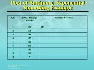
Example: Cod Catch • The Bay City Seafood Company recorded the monthly cod catch for the previous two years, as given below.
Example: Cod Catch • The plot of these data suggests that there is no trend or seasonal pattern. Therefore, a NO TREND model is suggested: It is also possible that the mean (or level) is slowly changing over time.
Example: Cod Catch • Step 1: Compute ℓ0 by averaging the first twelve time series values. Though there is no theoretical justification, it is a common practice to calculate initial estimates of exponential smoothing procedures by using HALF of the historical data.
Example: Cod Catch • Step 2: Begin with the initial estimate ℓ0 = 360.6667 and update it by applying the smoothing equation to the 24 observed cod catches. Set = 0.1 arbitrarily and judge the appropriateness of this choice of by the model’s in-sample fit.
Example: Cod Catch • Results associated with different values of
Example: Cod Catch • Step 3: Find a good value of that provides the minimum value for MSE (or SSE). • Use Solver in Excel as an illustration SSE alpha
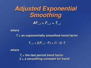
Holt’s Trend Corrected Exponential Smoothing • If a time series is increasing or decreasing approximately at a fixed rate, then it may be described by the LINEAR TREND model If the values of the parameters β0 and β1 are slowly changing over time, Holt’s trend corrected exponential smoothing method can be applied to the time series observations. Note: When neither β0 nor β1 is changing over time, regression can be used to forecast future values of yt. • Level (or mean) at time T: β0 + β1T Growth rate (or trend): β1
Holt’s Trend Corrected Exponential Smoothing • A smoothing approach for forecasting such a time series that employs two smoothing constants, denoted by and . • There are two estimates ℓT-1 and bT-1. • ℓT-1 is the estimate of the level of the time series constructed in time period T–1 (This is usually called the permanent component). • bT-1 is the estimate of the growth rate of the time series constructed in time period T–1 (This is usually called the trend component).
Holt’s Trend Corrected Exponential Smoothing • Level estimate • Trend estimate where = smoothing constant for the level (0 ≤ ≤ 1) = smoothing constant for the trend (0 ≤ ≤ 1)
Holt’s Trend Corrected Exponential Smoothing • Point forecast made at time T for yT+p • MSE and the standard error s at time T
Yt YT+1 T+1 T YT T - 1 T T + 1 T + 2
Procedures of Holt’s Trend Corrected Exponential Smoothing • Use the example of Thermostat Sales as an illustration
Procedures of Holt’s Trend Corrected Exponential Smoothing • Findings: • Overall an upward trend • The growth rate has been changing over the 52-week period • There is no seasonal pattern Holt’s trend corrected exponential smoothing method can be applied
Procedures of Holt’s Trend Corrected Exponential Smoothing • Step 1: Obtain initial estimates ℓ0 and b0 by fitting a least squares trend line to HALF of the historical data. • y-intercept = ℓ0; slope = b0
Procedures of Holt’s Trend Corrected Exponential Smoothing • Example • Fit a least squares trend line to the first 26 observations • Trend line • ℓ0 = 202.6246; b0 = – 0.3682
Procedures of Holt’s Trend Corrected Exponential Smoothing • Step 2: Calculate a point forecast of y1 from time 0 • Example
Procedures of Holt’s Trend Corrected Exponential Smoothing • Step 3: Update the estimates ℓT and bT by using some predetermined values of smoothing constants. • Example: let = 0.2 and = 0.1
Procedures of Holt’s Trend Corrected Exponential Smoothing • Step 4: Find the best combination of and that minimizes SSE (or MSE) • Example: Use Solver in Excel as an illustration SSE alpha gamma
Holt’s Trend Corrected Exponential Smoothing • p-step-ahead forecast made at time T • Example - In period 52, the one-period-ahead sales forecast for period 53 is • In period 52, the three-period-ahead sales forecast for period 55 is
Holt’s Trend Corrected Exponential Smoothing • Example • If we observe y53 = 330, we can either find a new set of (optimal) and that minimize the SSE for 53 periods, or • we can simply revise the estimate for the level and growth rate and recalculate the forecasts as follows:
Holt-Winters Methods • Two Holt-Winters methods are designed for time series that exhibit linear trend - Additive Holt-Winters method: used for time series with constant (additive) seasonal variations • Multiplicative Holt-Winters method: used for time series with increasing (multiplicative) seasonal variations • Holt-Winters method is an exponential smoothing approach for handling SEASONAL data. • The multiplicative Holt-Winters method is the better known of the two methods.
Multiplicative Holt-Winters Method • It is generally considered to be best suited to forecasting time series that can be described by the equation: • SNt: seasonal pattern • IRt: irregular component • This method is appropriate when a time series has a linear trend with a multiplicative seasonal pattern for which the level (β0+ β1t), growth rate (β1), and the seasonal pattern (SNt) may be slowly changing over time.
Multiplicative Holt-Winters Method • Estimate of the level • Estimate of the growth rate (or trend) • Estimate of the seasonal factor where , , and δ are smoothing constants between 0 and 1, L = number of seasons in a year (L = 12 for monthly data, and L = 4 for quarterly data)
Multiplicative Holt-Winters Method • Point forecast made at time T for yT+p • MSE and the standard errors at time T
Procedures of Multiplicative Holt-Winters Method • Use the Sports Drink example as an illustration
Procedures of Multiplicative Holt-Winters Method • Observations: • Linear upward trend over the 8-year period • Magnitude of the seasonal span increases as the level of the time series increases Multiplicative Holt-Winters method can be applied to forecast future sales
Procedures of Multiplicative Holt-Winters Method • Step 1: Obtain initial values for the level ℓ0, the growth rate b0, and the seasonal factors sn-3, sn-2, sn-1, and sn0, by fitting a least squares trend line to at least four or five years of the historical data. • y-intercept = ℓ0; slope = b0
Procedures of Multiplicative Holt-Winters Method • Example • Fit a least squares trend line to the first 16 observations • Trend line • ℓ0 = 95.2500; b0 = 2.4706
Procedures of Multiplicative Holt-Winters Method • Step 2: Find the initial seasonal factors • Compute for the in-sample observations used for fitting the regression. In this example, t = 1, 2, …, 16.
Procedures of Multiplicative Holt-Winters Method • Step 2: Find the initial seasonal factors • Detrend the data by computing for each time period that is used in finding the least squares regression equation. In this example, t = 1, 2, …, 16.
Procedures of Multiplicative Holt-Winters Method • Step 2: Find the initial seasonal factors • Compute the average seasonal values for each of the L seasons. The L averages are found by computing the average of the detrended values for the corresponding season. For example, for quarter 1,
Procedures of Multiplicative Holt-Winters Method • Step 2: Find the initial seasonal factors • Multiply the average seasonal values by the normalizing constant such that the average of the seasonal factors is 1. The initial seasonal factors are
Procedures of Multiplicative Holt-Winters Method • Step 2: Find the initial seasonal factors • Multiply the average seasonal values by the normalizing constant such that the average of the seasonal factors is 1. • Example CF = 4/3.9999 = 1.0000
Procedures of Multiplicative Holt-Winters Method • Step 3: Calculate a point forecast of y1 from time 0 using the initial values
Procedures of Multiplicative Holt-Winters Method • Step 4: Update the estimates ℓT, bT, and snT by using some predetermined values of smoothing constants. • Example: let = 0.2, = 0.1, and δ = 0.1