Download
1 / 28
280 likes | 389 Views
Determining Aggregate Demand (AD). This chapter -- looks at the components of Aggregate Expenditure. Examines the major causes of Consumption (C), Investment (I), Government Expenditure Net of Taxes (G - T), and Net Exports (X - M). Causes of Consumption (C).

E N D
Determining Aggregate Demand (AD) • This chapter -- looks at the components of Aggregate Expenditure. • Examines the major causes of Consumption (C), Investment (I), Government Expenditure Net of Taxes (G - T), and Net Exports (X - M).
Causes of Consumption (C) • Aggregate Income (Y), Y C • Wealth, Wealth C • Consumer Confidence (CC), CC C
Applying the Causes to Aggregate Demand (AD) • Aggregate Income (Y), appears on the graph, Y C relationship affects the shape of the AD curve. • Changes in Wealth or Consumer Confidence make up autonomous consumption (consumption due to causes other than Y) -- shift the AD curve.
Consumer Confidence and the Economy • Example -- effect of a decrease in consumer confidence. • CC C • Therefore the AD curve shifts leftward. • In the AD-AS model, this results in Y*, P*
Causes of Investment (I) The Capital Market • Investment (I) -- primarily business purchases of new plant and equipment along with new residential housing. • Large expenditures create the need for long-term borrowing. Borrowing is done from financial intermediaries such as banks or by companies issuing bonds or stock.
Investment and Capital Market Behavior • Investment results from behavior in the capital market. • The Capital Market -- the demand and supply for financial capital needed to finance purchases of plant and equipment (I).
The Demand For Financial Capital (DI) -- Major Causes • Nominal (Long-Term) Interest Rate (r) – cost of borrowing to finance investment r DI • Expected Inflation Rate (e) e DI • Business Confidence (BC) BC DI
Formalizing the Demand for Financial Capital (DI) • Graph DI against one of its causes -- the nominal interest rate (r). • Inverse relationship implies that the curve is downward sloping. • Changes in r are described as a movement along the curve. • Graph is drawn assuming that other causes are constant (ceteris paribus).
Shifts in the Demand for Financial Capital • Changes in causes other than r are described as shifts of the DI curve. • Changes that increase the Demand for Financial Capital shift the DI curve rightward. • Changes that decrease the Demand for Financial Capital shift the DI curve leftward.
The Supply of Financial Capital (SI) -- Major Causes • Nominal Interest Rate (r) r SI • Expected Inflation Rate (e) e SI • People’s Willingness to Save (S) S SI
Other Causes -- Supply of Financial Capital • Monetary Policy -- affects banks ability to loan (more later). • Foreigners’ willingness to buy US bonds or stock (Capital Flow). • Next Step -- Formalizing the above SI relationship
Formalizing the Supply of Financial Capital (SI) • Graph SI versus one of its causes -- the nominal interest rate (r). • Positive relationship implies that the curve is upward sloping. • Changes in r are described as a movement along the curve. • Graph is drawn assuming that other causes are constant (ceteris paribus).
Shifts in the Supply of Financial Capital • Changes in causes other than r are described as shifts of the SI curve. • Changes that increase the Supply of Financial Capital shift the SI curve rightward. • Changes that decrease the Supply of Financial Capital shift the SI curve leftward.
Equilibrium in the Capital Market -- Determining I • Investment (I*) occurs where the Demand for Financial Capital (DI) equals the Supply of Financial Capital (SI). • Shifts in the Demand or Supply of Financial Capital, as a result, change Investment (I*) • Because they change Investment, they also change Aggregate Demand, and Y*, and P* as a result.
Example 1 -- An Increase in Business Confidence (BC) • BC DI • DI curve shifts rightward I • Because investment increases, the AD curve shifts rightward. • In the AD-AS model, this results in Y*, P*.
Example 2 -- An Increase in Foreign Capital Flows to US • Capital Flow SI • SI curve shifts rightward I • Because investment increases, the AD curve shifts rightward. • In the AD-AS model, this results in Y*, P*.
Causes of (G - T) • Government Purchases of Goods and Services (G), Net Taxes (T), are policy variables. • Basically controlled by the government. • G, T changed for policy purposes (Fiscal Policy), other reasons as well.
Example -- War and the Economy • War Need for More Soldiers and Weapons G (G - T) • Because (G - T) increases, the AD curve shifts rightward. • In the AD-AS model, this results in Y*, P*.
Causes of Net Exports (NX) • General Principles -- NX = X - M, must consider causes of both exports and imports. -- Assume for simplicity that the world consists of 2 countries, the US and the rest of the world.
Specific Causes of Net Exports (NX = X - M) • World Output or Income (YW) YW X NX • US Output or Income (Y) Y M NX • Barriers to Trade (Tariffs, Quotas) • The Exchange Rate (e) e NX
A Digression -- Introduction to Exchange Rates • Exchange Rate (e) -- the amount of foreign currency needed to be exchanged for one (US) dollar. • Also known as the “value of the dollar”. • Conversion Ratio, in units of (foreign currency)/(US dollar)
Types of Exchange Rates • Bilateral Exchange Rates -- exchange rate between the US and an individual country. • Multilateral (Trade Weighted) Exchange Rate -- weighted average of bilateral exchange rates expressed as an index (macro measure of exchange rate).
Using Exchange Rates as a Conversion Ratio • Both Examples: US exchange rate vs Japanese Yen = 100 (yen/$). • Example 1 -- Suppose that dinner for two people in the US costs $50. Find its price in terms of yen. ($50)(100 yen) = 5000 yen (1 $)
Example 2 -- The Exchange Rate as a Conversion Ratio • Example 2 -- Suppose that dinner for two people in Japan costs 6832 yen. Find its price in terms of US dollars ($). (6832 yen) (1 $) = $68.32 (100 yen) • Note: e = 100 (yen/$)
Exchange Rate Changes e price of American goods and services to foreigners price of foreign goods and services to Americans e price of American goods and services to foreigners price of foreign goods and services to Americans
The Exchange Rate and Net Exports e (appreciating dollar, stronger dollar) X, M (X - M) e (depreciating dollar, weaker dollar) X, M (X - M)
Return to Aggregate Demand -- An Example • Example -- effect of a decrease in world output or income (YW). • YW X (X - M) • Therefore the AD curve shifts leftward. • In the AD-AS model, this results in Y*, P*
Aggregate Demand Changes and the Economy • Lots of factors shift aggregate demand (AD), affect Y* and P*. • Poses challenges: economy subject to “buffeting winds,” blows the economy off course (either to where Y* < YF or Y* > YF). • Role of Economic Policy -- to counteract “buffeting winds,” to take steps to move Y* closer to YF.