Download
1 / 115
1.15k likes | 1.28k Views
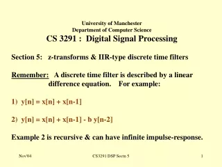
University of Manchester School of Computer Science Comp30291 Digital Media Processing 2007-08 Section 4 ‘Design of FIR digital filters’. x[n]. z -1. z -1. z -1. z -1. a M. a M-1. a 0. a 1. y[n]. 4.1.Introduction

E N D
University of Manchester School of Computer Science Comp30291 Digital Media Processing 2007-08 Section 4 ‘Design of FIR digital filters’ Comp30291: Section 4
x[n] ... z-1 z-1 z-1 z-1 aM aM-1 a0 a1 y[n] 4.1.Introduction FIR digital filter of order M implemented by programming the signal-flow-graph shown below. Its difference equation is: y[n] = a0x[n] + a1x[n-1] + a2x[n-2] + ... + aMx[n-M] Comp30291: Section 4
x[n] z-1 z-1 z-1 z-1 z-1 z-1 z-1 z-1 z-1 z-1 a0 a10 a1 a3 a4 a5 a6 a7 a8 a9 a2 + + + + + + + + + + y[n] 10th order FIR digital filter Comp30291: Section 4
Background, objective & methodology • Its impulse-response is {h[n]} = {..., 0, ..., a0, a1, a2,..., aM, 0, ...} • Taking DTFT of impulse-response gives the frequency-response: • Objective is to choose a0, a1,..., aM such that H(ej) is close to some target frequency-response H’(ej) ). • Inverse DTFT of H’(ej) gives required impulse-response : • Methodology is to use inverse DTFT to get an impulse- response {h[n]} & then realise some approximation to it. Comp30291: Section 4
Observations about the inverse-DTFT • It is an integral • It has complex numbers • Range of integration is from - to so it involves negative frequencies. Comp30291: Section 4
Reminder about integration x(t) t (Have +ve & ve areas) a b Comp30291: Section 4
Reminder about complex numbers • Let x = a + j.b, j = [-1] • Modulus: |x| = [a2 + b2] • Arg(x)=tan-1(b/a) + {.sign(b) if a < 0} = tan2(b,a) = angle(a + j.b) : range - to • Polar: x = Rej where R = |x| & = Arg(x) • De Moivre: ej = cos() + j.sin() • e-j = cos() - j.sin() • ej + e-j = 2cos() & ej - e-j = 2 j.sin() • Complex conjugate: x* = a - j.b = Re-j • That’s about it! Comp30291: Section 4
Bits of MATHs ea.eb = e(a+b) (ea)2 = e2a |A|.|B| = |A.B| but |A+B| |A| + |B| etc. Comp30291: Section 4
What about the negative frequencies? • Examine the DTFT formula for H(ej). • If h[n] real then h[n]ej is complex-conj of h[n]e-j. • Adding up terms gives H(e-j ) as complex conj of H(ej). • G() = G(-) since G() = |H(ej)| & G() = H(e-j)| • (Mod of a complex no. is Mod of its complex conj.) • (-) = () since() = Arg(H(ej)) & (-) = Arg(H(e-j)) • (Arg of a complex no. is Arg of its complex conj). Comp30291: Section 4
G() - 0 -() - Gain & phase response graphs with ve frequencies As G(-) = G(),gain-response is always symmetric about =0 As () = (),phase-response is always anti-symmetric about = 0 Comp30291: Section 4
G() 1 - /3 /3 0 4.2. Design of an FIR low-pass filter Assume we require lowpass filter whose gain-response approximates the ideal 'brick-wall' gain-response: If we take phase-response () = 0 for all , the required target frequency-response is: Comp30291: Section 4
By inverse DTFT, required impulse-response is: Comp30291: Section 4
To complete the calculation: Comp30291: Section 4
Graph of sinc(x) against x sinc(x) 1 Main ‘lobe’ ‘Ripples’ x -1 -3 -2 1 2 3 -4 ‘Zero-crossings’ at x =1, 2, 3, etc. Comp30291: Section 4
Plotting this ‘sinc’ graph in MATLAB clear all; close all; clc; x = [-10: 0.1 : 10]; y = sinc(x); figure(1); plot(x,y); grid on; title('sinc function'); xlabel( 'x'); ylabel('sinc(x)'); legend('sinc(x)', 'Location','Best'); axis([-10 10 -0.3 1]); Comp30291: Section 4
Graph of sinc(x) against x ‘Main lobe’ ‘Zero-crossings’ at x =1, 2, 3, etc ‘Ripples’ Comp30291: Section 4
Impulse-response for this ideal (brick-wall) lowpass filter Comp30291: Section 4
Plotting this ‘stem’ graph in MATLAB n=[-20:20]; h = (1/3)*sinc(n/3); figure(1); stem(n,h,'.:'); grid on; title('h[n] = (1/3) sinc(n/3)'); xlabel( 'n'); ylabel('h[n]'); legend('(1/3)sinc(n/3)', 'Location','Best'); axis([-20 20 -0.1 0.35]); for n=-20:20, disp(sprintf('n:%2d, h[n]: %6.3f' ,n,h(n+21))); end; Comp30291: Section 4
‘Ideal’ impulse-response • Reading from the graph or the MATLAB display, we get: • {h[n]} = { ..., -0.055, -0.07, 0, 0.14, 0.28, 0.33, 0.28, 0.14, 0, -0.07, -0.055, ... } • A digital filter with this impulse-response would have exactly the ideal frequency-response we applied to the inverse-DTFT. • ‘Brick-wall’ low-pass gain response & phase = 0 for all . • But {h[n]} has non-zero samples extending from n = - to , • Not a finite impulse-response. • Also not causal. • Not realisable in practice. Comp30291: Section 4
To produce a realisable impulse-response {h[n]}: Assume M is order of required filter & that M is even. (2) Delay resulting sequence by M/2 samples to ensure that the first non-zero sample occurs at n = 0. Step (1) is ‘truncation’ or ‘windowing’ Comp30291: Section 4
n Starting with ‘ideal’ impulse-response: h[n] = (1/3)sinc(n/3) Comp30291: Section 4
h[n] M=10 Truncate to M/2 n h[n] Delay by M/2 samples n Comp30291: Section 4
Causal & finite impulse-response • If M=10, finite impulse response obtained is: • { ...0, -0.055, -0.07, 0, 0.14, 0.28, 0.33, 0.28, 0.14, 0, -0.07, -0.055, 0... } • Obtained by truncating & delaying {h[n]} for ‘ideal’ lowpass digital filter with cut-off /3 radians/sample. • Taking M = 4, we would obtain: • {.., 0, .., 0, 0.14, 0.28, 0.33 , 0.28 , 0.14 , 0 ,..,0,..} • Resulting causal impulse-response now realised by setting: • an = h[n] for n = 0,1,2,...,M. Comp30291: Section 4
x[n] -1 z-1 z-1 z z-1 a4 a3 a1 a0 a2 0.14 0.28 0.33 0.28 0.14 + y[n] FIR filter realisation (M=4) ( Note:4th order FIR filter has 4 delays & 5 multipliers ). • Gain & phase responses may be derived by MATLAB. Comp30291: Section 4
-6dB -21 dB Gain dropsto - dB /3 Fs/6 FC Fs/2 Straight line Jumpsby 180O Plot gain & phase responses of 4th order FIR filter Comp30291: Section 4
MATLAB prog for truncating & plotting gain & phase n=[-20:20]; h = (1/3)*sinc(n/3); M=4; % FIR filter order Fs = 8000; % Sampling freq (Hz) for n=-M/2 : M/2 a(n + M/2 + 1) = h(n+21); end; figure(1); freqz(a,1,200,Fs); Comp30291: Section 4
20 -6dB 0 -21 dB -20 Gain dropsto - dB Magnitude (dB) -40 Fs/2 -60 0 500 1000 1500 2000 2500 3000 3500 4000 /3 Fs/6 FC Frequency (Hz) Gain-response of 4th order FIR filter (zoomed) • Gain starts at 0 dB in pass-band & falls to -6 dB at cut-off frequency. • There are two ‘stop-band ripples’ & gain is -21 dB at peak of first. Comp30291: Section 4
Phase-lag 2 300O 200 100 Fs/2 /2 F Hz 0 1000 FC 2000 3000 4000 Phase-lag response of 4th order FIR filter • Linear phase in pass-band • Don’t worry about 180 degree jumps in stop-band for now. Comp30291: Section 4
() - -() - Why do we not get a zero phase-response? • We started by specifying that phase = 0 for all . • We ended up with a phase-response as follows: Only pass-band part is shown here • Phase response affected by the delay of M/2 samples. Comp30291: Section 4
Estimation of phase-delay from slope • For a linear phase LTI system, -() / is ‘phase-delay’ in sampling intervals. • Look at phase-response graph in pass-band. • Phase decreases by 180o in 2000Hz (Fs = 8000 Hz) • radians in /2 radians/second • -() / /2 = 2 sampling intervals • So the phase-delay is 2. • Not a surprise as we delayed the impulse-response by 2 samples to make it causal (M=4). Comp30291: Section 4
Using MATLAB functions ‘fir1’ & ‘freqz’ • Same result obtained using ‘fir1’ as follows: c = fir1(4, 0.33, rectwin(5), 'noscale'); • Reason for rectwin(5) & ‘noscale’ will be clear later. • To plot gain & phase response: freqz(c, 1, 500, Fs); • Plots 500 points & frequency-axis to range 0-Fs/2 !! • Plots () against rather than phase lag -(). • Phase ‘unwrapped’ to avoid 360o jumps. Comp30291: Section 4
Gain & phase responses of 4th order FIR filter by MATLAB Comp30291: Section 4
Effect of truncating {h[n]} to M/2 & delaying by M/2 samples • Gain & phase responses different from those originally specified. • Gain-response: cut-off rate not ‘brick-wall’, • 0 dB at 0 Hz & drops to -6 dB at cut-off frequency, • ‘ripples’ and ‘zeros’ appear in stop-band, • peak of the first ripple at about -21dB. • Phase-response: not zero for all as originally specified, • linear phase in pass-band • -( )/ = M/2 for | | /3; • phase-delay = M/2 sampling intervals. • Jumps of 180o occur in stop-band. • Jumps of 360o avoided by unwrapping. Comp30291: Section 4
Can we improve low-pass filter by increasing order to ten? • Taking 11 terms of { (1/3)sinc(n/3)} we get, • after delaying by 5 samples: • {...0,-0.055,-.069, 0,.138,.276,.333,.276,.138,0,-.069,-.055,0,...}. • To obtain same result from MATLAB7: • c = fir1(10, 0.33, rectwin(11), 'noscale'); • freqz(c); Comp30291: Section 4
x[n] z-1 z-1 z-1 z-1 z-1 z-1 z-1 z-1 z-1 z-1 0 -.07 -.07 .28 .28 0.14 0 -.055 0.14 .33 -.055 + + + + + + + + + + y[n] 10th order FIR digital lowpass filter(/3 rect) The coeffs are symmetric because the filter is linear phase. Comp30291: Section 4
For 10th order low-pass filter with C = /3: Comp30291: Section 4
Gain & phase responses of 20th order lowpass FIR filter with C = /3 Comp30291: Section 4
Gain & phase responses of 60th order lowpass FIR filter with C = /3 Comp30291: Section 4
Gain & phase of 100th order low-pass FIR filter with C = /3 Comp30291: Section 4
Gain-response of 10th order lowpass FIR filter with WC = /3 Comp30291: Section 4
Gain response of 20th order lowpass FIR filter with WC = /3 Comp30291: Section 4
Effect of increasing order on gain & phase responses • Cut-off rate increases as order (M) increases. • Number of stop-band ripples increases with order. • Gain at peak of first ripple after cut-off remains at -21 dB. • Remains exactly ‘linear phase’ in pass-band but slope of phase-response (=phase-delay) increases since -() / = M/2. • NB: freqz ‘unwraps’ phase-response avoiding 360o jumps! • Filter not really improving with increasing order. • To improve matters we need to discuss ‘windowing’. Comp30291: Section 4
rM[n] n -M/2 M/2 4.3. Windowing By truncating {h[n]} for ideal filter, we effectively multiplied {h[n]} by a rectangular window sequence {rM[n]} to produce {h[n]} where Comp30291: Section 4
Effect of rectangular window on freq-response • Sudden transitions to zero at rectangular window edges cause the stop-band ripples we saw in the gain-response graphs. • Why is this? Consider DTFT of {rM[n]} when 0, 2, ... Comp30291: Section 4
DTFT of rect-window {rM[n]} When = 0, RM(ej) = M+1 • Shows RM(ej) for M=20 • Purely real. • Looks a bit like sinc. • Has main-lobe & ripples. • Ripples cause stop-band ripples in gain-resp Comp30291: Section 4
MATLAB program to plot RM(ej) M = 20; W = -3.2 : 0.001 : 3.2; if W==0, R=M+1; else R=sin((M+1)*W/2)./sin(W/2); end; figure(1); plot(W,R); grid on; title(sprintf('Dirichlet K of order %d ', M)); axis([-3.2 3.2 -M*0.3 M+2]); xlabel('radians/sample'); ylabel('R'); Comp30291: Section 4
Frequency-domain convolution • Multiplying two sequences {x[n]} & {[y[n]} to produce {x[n].y[n]} is called ‘time-domain multiplication’. • It may be shown* that if {x[n]} has DTFT X(ej) & [y[n]} has DTFT Y(ej) then the DTFT of {x[n].y[n]} is: • Time-domain multiplication is equivalent to frequency-domain convolution. *Appendix B Comp30291: Section 4
Apply this formula to rectangular window • Multiplying an ideal impulse resp {h[n]} by the rect window {rM[n]} causes H(ej) to be ‘convolved’ with RM(ej). • If H(ej) has ideal brick-wall gain-response, & RM(ej) is as shown in previous graph, convolving H(ej) with RM(ej) reduces cut-off rate & introduces stop-band ripples. • The sharper the main-lobe of RM(ej) and the lower the ripples, the better. Comp30291: Section 4
Illustration for ideal /3 lowpass filter • What happens to area under curve as increases from 0 to ? Comp30291: Section 4
=0 Area under curve /3 to +/3: 1 /3 /3 Comp30291: Section 4