Download
1 / 44
440 likes | 446 Views
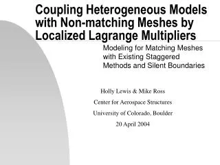
Coupling Heterogeneous Models with Non-matching Meshes. Modeling for Matching Meshes with Existing Staggered Methods and Silent Boundaries. Mike Ross Center for Aerospace Structures University of Colorado, Boulder 24 February 2004. Topics of Discussion. Introduction of the Research Topic

E N D
Coupling Heterogeneous Models with Non-matching Meshes Modeling for Matching Meshes with Existing Staggered Methods and Silent Boundaries Mike Ross Center for Aerospace Structures University of Colorado, Boulder 24 February 2004
Topics of Discussion • Introduction of the Research Topic • Benefits • Plan of Attack for this Research • Progress (Benchmark Model) • Direction for the Future
Why am I Here??? • NSF Grant • PIs: Professor Felippa & Professor Park • Crux: Model different physical systems with non-matching meshes • Use existing models of individual physical systems. • Develop interaction techniques for different models • with use of a localized connection frames and localized multipliers.
Application Drivers • MEMS Device (Mechanical Eng.) • Electrical-Mechanical-Thermal Interaction • Dam under seismic excitation (Civil Eng.) • Fluid-Structure-Soil Interaction • Reason: • NSF granting division is Civil & Mechanical systems (CMS)
A Picture is Worth 1,000 Words Multi-physic system Modular Systems Connected by Localized Interaction Technique (Black Lines)
Benefits/Goals: • Maintain software modularity through an interface frame • Provides great flexibility for different FEM Codes, etc. • Custom discretizations and solvers for different physics • Simplify the treatment of non-matching meshes • Efficient high fidelity simulation • Meaning: resources can be put on critical parts of the problem • User Friendly
Plan of Attack • Generate a benchmark model • Use current available methods • Matching meshes • Generate a model with localized frames • Maintain matching meshes • Generate a model with localized frames • With nonmatching meshes
Current Progress (Benchmark Model) Dam (Brick Elements) Fluid (Spectral Elements) Soil (Brick Elements) • Output: Displacements of Dam & Cavitation Region • Assume: Plane Strain (constraints reduce DOF) • Only looking at seismic excitation in the x-direction • Linear elastic brick elements
Benchmark Concept:Staggered Method with Non-Reflecting Boundary displacements pressures Structure (seismic displacement) Non-Reflecting Boundary (NRB) Fluid Volume pressures displacements
Structure Equations: • x = relative displacements • Acceleration (a) is from Berkeley’s PEER database • Damping modeled with Rayleigh damping • Solved with a Central Difference Method (Explicit). Easy to implement. Also the physics can be represented with small time steps • Silent Boundary on Soil is modeled with a Viscous Damping Boundary Method • Soil and Dam are modeled monolithically with different properties (i.e. Young’s Modulus, etc.)
Relative Displacement Concept Summation of Forces: Matrix Form:
Relative Displacement Concept Define Relative Displacements Insert into summation of forces equation Matrix Form Key to remember is that total displacement = earthquake displacement - relative displacement
Central Difference Expand Xn+1 & Xn-1 in Taylor Series about time n t Ignore higher order terms and add and subtract (1) & (2) to yield. Insert these two into the EOM The Central Difference is said to be second-order accurate. Halving the time step should approximately quarter the error.
Stability of Uncoupled Structural Time Integration • Central Difference is conditionally stable (General for explicit methods). • By going through a Fourier/Spectral Stability: • For propagating waves: • CFL condition: • t must be small enough that information does not propagate across more than one element per time step.
JOKE TIME A football player and an engineer are applying for the same job. The boss said, “Boys, you need to take a test before you can get this job. So they took the test and the next day they came back to see who the boss chose. “Well,” he said, “Both of you got the same score except I’m going to choose the engineer.” The football player complained, “Don’t you think that’s prejudice or something?” “Well,” the boss said,”Let me tell you what happened. Both of your papers were right all the way through until the last question came up, and the engineer answered ‘I don’t know’ and then when I looked at your paper, you answered, ‘Me either’”.
Fluid Equations: • Assumptions • Fluid is inviscid & irrotational • Displacements are small; thus, density is constant • Fluid is compressible with a bulk modulus • Bilinear acoustic fluid (bilinear to account for cavitation) • Fluid cannot transmit negative pressures • System is initial in static equilibrium • Steady body force field (gravity) • Goal is to develop continuum fluid models that are discretized with the spectral-element method.
Fluid: Momentum Equation Definitions for Fluid Volume Force is conservative with Potential Energy Newton’s Law (F = ma). Momentum Equation
Fluid: Momentum Equation Compare to Euler’s Equation For an acoustic fluid starting at rest one can assume the following in the acceleration term: Thus,
Fluid: Displacement Potential Because fluid motion is assumed irrotational, the displacement field can be expressed in terms of the gradient of a scalar function (x,y,z,t). Check Irrotational Condition:
Fluid: Equation of Motion Replace acceleration term with this displacement potential in the Momentum Equation. Spatial Integrate:
Fluid: Equation of Motion At Static Equilibrium: EOM
Fluid: Constitutive Equation • For a linear acoustic fluid: • K = fluid Bulk Modulus • Property to Characterize Compressibility • Increase Pressure -> Decrease Volume • K = c2; c = speed of sound of the medium. • Define ‘Densified Relative Condensation’ • Insert: K = c2 & Into Constitutive Eqn. Constitutive Eqn.
Fluid: Governing Equation • Compare EOM and the Constitutive Equations: • We see the following : • Apply the wave equation for a Linear Fluid: • Get the Governing Equation:
Fluid Equations: (Spectral Elements) • Dependent field Variables representation within each element • Essences of Spectral Elements is the choice of & quadrature rule • by Lagrangian Interpolants with Gauss-Lobatto-Legendre (GLL) quadrature points. • Element-node locations are coincident with the quadrature points Standard Gauss Quadrature 1-D GLL Quadrature 1-D Linear Shape functions -1 1 -1 1 Locations -1/(3) 1/(3) -1 1
Fluid Equations: • Discretize governing equation with Galerkin approach • Apply Green’s first formula • Insertion of dependent field variable representation, yields the element-level algebraic equations.
Fluid Equations: • Assemble into global system • Q : Capacitance Matrix with Spectral elements (becomes diagonal matrix) • H : Reactance Matrix • b : boundary-interaction vector • Explicit time integration to solve for s then solve for p
Fluid: Bilinear (Cavitation) • Cavitation is the spontaneous vaporization of a fluid. It happens when the fluid pressure < vapor pressure. • Water’s vapor pressure << atmospheric pressure • Simple Mathematical model is that if the total pressure is negative then it is just zero.
Explicit Integration for Fluid • = dimensionless damping coefficient (varies from 0 to 1) • Add numerical damping to the EOM to reduce frothing • Modified Solution Advance Process with Cavitation • Insert into Main Fluid Equation: • bn+1 is from predicted structure and NRB displacements • Solve Linear system for sn+1, Remember Q is diagonal
Stability of Uncoupled Fluid Time Integration • Fourier Stability Analysis • see Felippa, Deruntz, sec. 2.4 • is the eigenvalue of (H- Q)z=0. • Gerschgorin’s theorem can be used to obtain an upper bound on max.
Time for a little laughter: “Outside of the killings, Washington has one of the lowest crime rates in the country,” - Washington DC mayor Marion Barry “I’m not going to have some reporters pawing through out papers. We are the President,” - Hillary Clinton “It isn’t the pollution that’s harming the environment. It’s the impurities in our air and water that are doing it.” - Al Gore “It’s no exaggeration to say that the undecided could go one way or another” - George Bush
Coupling Temporal integration • NRB: • Structure Forcing: • Fluid Forcing:
Time Stepping: S S up Etc. F F tn tn+1
Time Stepping:Staggered Method add subcycling Example: Structure time = t; Fluid time = 2t; Subcycling = 2 S S S pb Etc. pn+2 up F F tn tn+1 tn+2
Time Stepping:Staggered Method add subcycling Example: Structure time = t; Fluid time = 2t; Subcycling = 2 New u start pressure Structure (seismic displacement, d) Non-Reflecting Boundary (NRB) Fluid Volume displacements pn+2 • Used Subcycling to reduce computational time and have the time increments near the upper bound of the stable time region for the fluid and the structure. Using a Euler Scheme for the prediction.
Subcycling • Trying to integrate the different systems with their critical time for stability • Critical time (fluid,3.5e-3 sec.)>(structure,2.5e-4 sec.) • We predict fluid displacements with Euler Scheme. Comparison of deflections with subcycling and without. Dam Crest Movement without subcycling Dam Crest Movement with subcycling
Output for Dam Crest Under Seismic Load no Soil With Fluid Interaction Without Fluid Interaction
Output for Dam Crest Under Seismic Load Soil Total Displacement of Dam Crest Relative Displacement of Dam Crest
Localized Frame Concept • Frames are connected to adjacent partitions by force/flux fields • Mathematically: Lagrange multipliers “gluing” the state variables of the partition models to that of the frame. • Lagrange multipliers at the frame are related by interface constraints and obey Newton’s Third Law.
Example of Localized Lagrange multipliers (Two-spring system) Subsystems Subsystem Energy Expressions (Variational Formulation)
Example of Localized Lagrange multipliers (Con’t) The physically represent the interface forces Identify Interface Constraints Total Virtual Work = 0 ( Stationary)
Example of Localized Lagrange multipliers (Con’t) Equations of Motion • Comments: • Notice the localized multipliers (Lagrange) • u1 = uf & u2 = uf (constraint) • Last row states that the sum of reaction forces at a node disappear when partitioned nodes are assembled (Newton’s third law) • This is just the set up for the transient interaction analysis.
Set Sail for the Future • Develop structure-fluid interaction via localized interfaces with nonmatching meshes. • Develop structure-soil interaction via localized interfaces spanning a range of soil media. • Develop a localized interface for cavitating fluid and linear fluid. • Develop rules for multiplier and connector frame discretization. • Implement and asses the effect of dynamic model reduction techniques.
Acknowledgments • NSF Grant CMS 0219422 • Professor Felippa & Professor Park • Mike Sprague (Professor Geer’s Ph.D student, now a post-doc in APPM) • CAS (Center for Aerospace Structures) CU