Download
1 / 41
420 likes | 576 Views
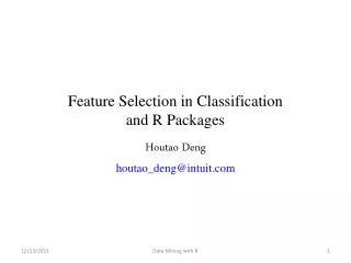
Feature selection, SVM-based classification and application to mass spectrometry data analysis. Elena Marchiori Department of Computer Science Vrije Universiteit Amsterdam. Overview. Support Vector Machines Variable selection Application in Bioinformatics. Support Vector Machines.

E N D
Feature selection, SVM-based classification and application to mass spectrometry data analysis Elena Marchiori Department of Computer Science Vrije Universiteit Amsterdam
Overview • Support Vector Machines • Variable selection • Application in Bioinformatics
Support Vector Machines • Advantages: • maximize the margin between two classes in the feature space characterized by a kernel function • are robust with respect to high input dimension • Disadvantages: • difficult to incorporate background knowledge • Sensitive to outliers
SVM • To construct optimal hyperplane • Minimize • Subject to • Constrained Optimization problem with Lagrangian
SVM • Primal variables vanish • KKT condition • Support Vectors whose is nonzero • Optimization problem • Maximize • Subject to • Decision function
ρ SVM: separable classes Support vectors uniquely characterize optimal hyper-plane margin Optimal hyper-plane Support vector
SVM and outliers outlier
Soft Margin Classification • What if the training set is not linearly separable? • Slack variablesξican be added to allow misclassification of difficult or noisy examples. ξj ξk
Weakening the constraints Weakening the constraints Allow that the objects do not strictly obey the constraints Introduce ‘slack’-variables
SVC with slacks The optimization problem changes into:
Tradeoff parameter C Notice that the tradeoff parameter C has to be defined beforehand. It weighs the contributions between the training error and the structural error. Its value is often optimized using cross-validation.
Influence of C Erroneous objects can still have a (large) influence on the solution
Classifying new examples • Once the parameters (*, b*) are found by solving the required quadratic optimisation on the training set of points, the SVM is ready to be used for classifying new points. • Given new point x, its class membership is sign[f(x, *, b*)], where Data enters only in the form of dot products!
x 0 x 0 Non-linear SVMs • Datasets that are linearly separable with some noise work out great: • But what are we going to do if the dataset is just too hard? • How about… mapping data to a higher-dimensional space: x2 x 0
Non-linear SVMs: Feature Spaces • Map the original feature space to some higher-dimensional feature space where the training set is separable: Φ: x→φ(x)
The “Kernel Trick” • The linear classifier relies on inner product between vectors K(xi,xj)=xiTxj • If every datapoint is mapped into high-dimensional space via some transformation Φ: x→φ(x), the inner product becomes: K(xi,xj)= φ(xi)Tφ(xj) • A kernel function is some function that corresponds to an inner product in some expanded feature space. • Example: 2-dimensional vectors x=[x1 x2]; let K(xi,xj)=(1 + xiTxj)2, Need to show that K(xi,xj)= φ(xi)Tφ(xj): K(xi,xj)=(1 + xiTxj)2,= 1+ xi12xj12 + 2 xi1xj1xi2xj2+ xi22xj22 + 2xi1xj1 + 2xi2xj2= = [1 xi12 √2 xi1xi2 xi22 √2xi1 √2xi2]T [1 xj12 √2 xj1xj2 xj22 √2xj1 √2xj2] = = φ(xi)Tφ(xj), where φ(x) = [1 x12 √2 x1x2 x22 √2x1 √2x2]
Examples of kernels • Example1: 2D input space, 3D feature space • Example2: in this case the dimension of is infinite • Note: Not every function is a proper kernel. There is a theorem called Mercer Theorem that characterises proper kernels • To test a new input x when working with kernels
SVM applications • SVMs were originally proposed by Boser, Guyon and Vapnik in 1992 and gained increasing popularity in late 1990s. • SVMs are currently among the best performers for a number of classification tasks ranging from text to genomic data. • SVM techniques have been extended to a number of tasks such as regression [Vapnik et al. ’97], principal component analysis [Schölkopf et al. ’99], etc. • Most popular optimization algorithms for SVMs are SMO [Platt ’99] and SVMlight[Joachims’ 99], both use decomposition to hill-climb over a subset of αi’s at a time. • Tuning SVMs remains a black art: selecting a specific kernel and parameters is usually done in a try-and-see manner.
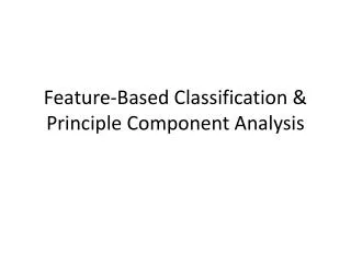
Variable Selection • Select a subset of “relevant” input variables • Advantages: • it is cheaper to measure less variables • the resulting classifier is simpler and potentially faster • prediction accuracy may improve by discarding irrelevant variables • identifying relevant variables gives more insight into the nature of the corresponding classification problem (biomarker detection)
Approaches • Wrapper • feature selection takes into account the contribution to the performance of a given type of classifier • Filter • feature selection is based on an evaluation criterion for quantifying how well feature (subsets) discriminate the two classes • Embedded • feature selection is part of the training procedure of a classifier (e.g. decision trees)
SVM-RFE: wrapper • Recursive Feature Elimination: • Train linear SVM -> linear decision function • Use absolute value of variable weights to rank variables • Remove half variables with lower rank • Repeat above steps (train, rank, remove) on data restricted to variables not removed • Output: subset of variables
SVM-RFE • Linear binary classifier decision function • Recursive Feature Elimination (SVM-RFE) • at each iteration: • eliminate threshold% of variables with lower score • recompute scores of remaining variables
SVM-RFE I. Guyon et al., Machine Learning, 46,389-422, 2002
RELIEF: filter • Idea: relevant variables make nearest examples of same class closer and make nearest examples of opposite classes more far apart. • Algorithm RELIEF: • Initialize weights of variables to zero. • For all examples in training set: • find nearest example from same (hit) and opposite class (miss) • update weight of variable by adding abs(example - miss) -abs(example - hit) • Rank variables using weights
Application in Bioinformatics Biomarker detection with Mass Spectrometric data of mixed quality
What does a mass spectrometer do? 1. It measures mass better than any other technique. 2. It can give information about chemical structures. What are mass measurements good for? To identify, verify, and quantitate: metabolites, recombinant proteins, proteins isolated from natural sources, oligonucleotides, drug candidates, peptides, synthetic organic chemicals, polymers Slides from University of California San Francisco
Applications of Mass Spectrometry • Pharmaceutical analysis • Bioavailability studies • Drug metabolism studies, pharmacokinetics • Characterization of potential drugs • Drug degradation product analysis • Screening of drug candidates • Identifying drug targets • Biomolecule characterization • Proteins and peptides • Oligonucleotides • Environmental analysis • Pesticides on foods • Soil and groundwater contamination • Forensic analysis/clinical Slides from University of California San Francisco
Summary: acquiring a mass spectrum Ionization Mass Sorting (filtering) Detection Ion Source Ion Detector Mass Analyzer • Form ions • (charged molecules) Sort Ions by Mass (m/z) • Detect ions 100 75 Inlet • Solid • Liquid • Vapor 50 25 0 1330 1340 1350 Mass Spectrum Slides from University of California San Francisco
MALDI: Matrix Assisted Laser Desorption Ionization Sample plate Laser hn • 1. Sample is mixed with matrix (X) and dried on plate. • 2. Laser flash ionizes matrix molecules. • 3. Sample molecules (M) are ionized by proton transfer: XH+ + M MH+ + X. MH+ Grid (0 V) +/- 20 kV Slides from University of California San Francisco
Time-of-flight (TOF) Mass Analyzer Source Drift region (flight tube) + + detector + + V • Measures the time for ions to reach the detector. • Small ions reach the detector before large ones. Slides adapted from University of California San Francisco
40000 30000 20000 10000 0 The mass spectrum shows the results MALDI TOF spectrum of IgG MH+ Relative Abundance (M+2H)2+ (M+3H)3+ 50000 100000 150000 200000 Mass (m/z) Slides from University of California San Francisco
Dataset • MALDI-TOF data. • samples of mixed quality due to different storage time. • controlled molecule spiking used to generate two classes.
Comparison of ML algorithms • Feature selection + classification: • RFE+SVM • RFE+kNN • RELIEF+SVM • RELIEF+kNN
LOOCV results • Misclassified samples are of bad quality (higher storage time) • The selected features do not always correspond to m/z of spiked molecules
LOOCV results • The variables selected by RELIEF correspond to the spiked peptides • RFE is less robust than RELIEF over LOOCV runs and selects also “irrelevant” variables RELIEF-based feature selection yields results which are better interpretable than RFE
BUT... • RFE+SVM yields superior loocv accuracy than RELIEF+SVM • RFE+kNN superior accuracy than RELIEF+kNN (perfect LOOCV classification for RFE+1NN) RFE-based feature selection yields better predictive performance than RELIEF
Conclusion • Better predictive performance does not necessarily correspond to stability and interpretability of results • Open issues: • how to measure reliability of potential biomarkers identified by feature selection algorithms? • Is stability of feature selection algorithms more important than predictive accuracy?