Download
1 / 41
410 likes | 529 Views
NAMD: Biomolecular Simulation on Thousands of Processors. James C. Phillips Gengbin Zheng Sameer Kumar Laxmikant Kale http://charm.cs.uiuc.edu Parallel Programming Laboratory Dept. of Computer Science And Theoretical Biophysics Group Beckman Institute

E N D
NAMD: Biomolecular Simulation on Thousands of Processors James C. Phillips Gengbin Zheng Sameer Kumar Laxmikant Kale http://charm.cs.uiuc.edu Parallel Programming Laboratory Dept. of Computer Science And Theoretical Biophysics Group Beckman Institute University of Illinois at Urbana Champaign
Funding Agencies NIH NSF DOE (ASCI center) Students and Staff Parallel Programming Laboratory Orion Lawlor Milind Bhandarkar Ramkumar Vadali Robert Brunner Theoretical Biophysics Klaus Schulten, Bob Skeel Coworkers PSC Ralph Roskies Rich Raymond Sergiu Sanielivici Chad Vizino Ken Hackworth NCSA David O’Neal Acknowledgements
NAMD: A Production MD program NAMD • Fully featured program • NIH-funded development • Distributed free of charge (~5000 downloads so far) • Binaries and source code • Installed at NSF centers • User training and support • Large published simulations (e.g., aquaporin simulation featured in keynote)
Acquaporin Simulation NAMD, CHARMM27, PME NpT ensemble at 310 or 298 K 1ns equilibration, 4ns production Protein: ~ 15,000 atoms Lipids (POPE): ~ 40,000 atoms Water: ~ 51,000 atoms Total: ~ 106,000 atoms 3.5 days / ns - 128 O2000 CPUs 11 days / ns - 32 Linux CPUs .35 days/ns–512 LeMieux CPUs F. Zhu, E.T., K. Schulten, FEBS Lett.504, 212 (2001) M. Jensen, E.T., K. Schulten, Structure9, 1083 (2001)
Molecular Dynamics in NAMD • Collection of [charged] atoms, with bonds • Newtonian mechanics • Thousands of atoms (10,000 - 500,000) • At each time-step • Calculate forces on each atom • Bonds: • Non-bonded: electrostatic and van der Waal’s • Short-distance: every timestep • Long-distance: using PME (3D FFT) • Multiple Time Stepping : PME every 4 timesteps • Calculate velocities and advance positions • Challenge: femtosecond time-step, millions needed! Collaboration with K. Schulten, R. Skeel, and coworkers
Sizes of Simulations Over Time BPTI 3K atoms ATP Synthase 327K atoms (2001) Estrogen Receptor 36K atoms (1996)
Easy Tiny working data Spatial locality Uniform atom density Persistent repetition Multiple timestepping Hard Sequential timesteps Short iteration time Full electrostatics Fixed problem size Dynamic variations Multiple timestepping! Parallel MD: Easy or Hard?
Other MD Programs for Biomolecules • CHARMM • Amber • GROMACS • NWChem • LAMMPS
Traditional Approaches: non isoefficient • Replicated Data: • All atom coordinates stored on each processor • Communication/Computation ratio: P log P • Partition the Atoms array across processors • Nearby atoms may not be on the same processor • C/C ratio: O(P) • Distribute force matrix to processors • Matrix is sparse, non uniform, • C/C Ratio: sqrt(P) Not Scalable
Spatial Decomposition • Atoms distributed to cubes based on their location • Size of each cube : • Just a bit larger than cut-off radius • Communicate only with neighbors • Work: for each pair of nbr objects • C/C ratio: O(1) • However: • Load Imbalance • Limited Parallelism Charm++ is useful to handle this Cells, Cubes or“Patches”
Virtualization: Object-based Parallelization User is only concerned with interaction between objects System implementation User View
Data driven execution Scheduler Scheduler Message Q Message Q
Charm++ Parallel C++ Asynchronous methods In development for over a decade Basis of several parallel applications Runs on all popular parallel machines and clusters AMPI A migration path for MPI codes Allows them dynamic load balancing capabilities of Charm++ Minimal modifications to convert existing MPI programs Bindings for C, C++, and Fortran90 Charm++ and Adaptive MPIRealizations of Virtualization Approach Both available from http://charm.cs.uiuc.edu
Software Engineering Number of virtual processors can be independently controlled Separate VPs for modules Message Driven Execution Adaptive overlap Modularity Predictability: Automatic Out-of-core Dynamic mapping Heterogeneous clusters: Vacate, adjust to speed, share Automatic checkpointing Change the set of processors Principle of Persistence: Enables Runtime Optimizations Automatic Dynamic Load Balancing Communication Optimizations Other Runtime Optimizations Benefits of Virtualization More info: http://charm.cs.uiuc.edu
Measurement Based Load Balancing • Principle of persistence • Object communication patterns and computational loads tend to persist over time • In spite of dynamic behavior • Abrupt but infrequent changes • Slow and small changes • Runtime instrumentation • Measures communication volume and computation time • Measurement based load balancers • Use the instrumented data-base periodically to make new decisions
Spatial Decomposition Via Charm • Atoms distributed to cubes based on their location • Size of each cube : • Just a bit larger than cut-off radius • Communicate only with neighbors • Work: for each pair of nbr objects • C/C ratio: O(1) • However: • Load Imbalance • Limited Parallelism Charm++ is useful to handle this Cells, Cubes or“Patches”
Object Based Parallelization for MD: Force Decomposition + Spatial Decomposition • Now, we have many objects to load balance: • Each diamond can be assigned to any proc. • Number of diamonds (3D): • 14·Number of Patches
New Challenges • New parallel machine with faster processors • PSC Lemieux • 1 processor performance: • 57 seconds on ASCI red to 7.08 seconds on Lemieux • Makes is harder to parallelize: • E.g. larger communication-to-computation ratio • Each timestep is few milliseconds on 1000’s of processors • Incorporation of Particle Mesh Ewald (PME)
F1F0 ATP-Synthase (ATP-ase) The Benchmark • CConverts the electrochemical energy of the proton gradient into the mechanical energy of the central stalk rotation, driving ATP synthesis (G = 7.7 kcal/mol). 327,000 atoms total, 51,000 atoms -- protein and nucletoide 276,000 atoms -- water and ions
NAMD Parallelization using Charm++ 700 VPs 9,800 VPs These 30,000+ Virtual Processors (VPs) are mapped to real processors by charm runtime system
Grainsize and Amdahls’s law • A variant of Amdahl’s law, for objects: • The fastest time can be no shorter than the time for the biggest single object! • Lesson from previous efforts • Splitting computation objects: • 30,000 nonbonded compute objects • Instead of approx 10,000
NAMD Parallelization using Charm++ 700 VPs 30,000 VPs These 30,000+ Virtual Processors (VPs) are mapped to real processors by charm runtime system
Distribution of execution times of non-bonded force computation objects (over 24 steps) Mode: 700 us
Load Balancing Steps Regular Timesteps Detailed, aggressive Load Balancing Instrumented Timesteps Refinement Load Balancing
Another New Challenge • Jitter due small variations • On 2k processors or more • Each timestep, ideally, will be about 12-14 msec for ATPase • Within that time: each processor sends and receives : • Approximately 60-70 messages of 4-6 KB each • Communication layer and/or OS has small “hiccups” • No problem until 512 processors • Small rare hiccups can lead to large performance impact • When timestep is small (10-20 msec), AND • Large number of processors are used
With barrier: Without: Benefits of Avoiding Barrier • Problem with barriers: • Not the direct cost of the operation itself as much • But it prevents the program from adjusting to small variations • E.g. K phases, separated by barriers (or scalar reductions) • Load is effectively balanced. But, • In each phase, there may be slight non-determistic load imbalance • Let Li,j be the load on I’th processor in j’th phase. • In NAMD, using Charm++’s message-driven execution: • The energy reductions were made asynchronous • No other global barriers are used in cut-off simulations
migrate Compute(s) away in this step Substep Dynamic Load Adjustments • Load balancer tells each processor its expected (predicted) load for each timestep • Each processor monitors its execution time for each timestep • after executing each force-computation object • If it has taken well beyond its allocated time: • Infers that it has encountered a “stretch” • Sends a fraction of its work in the next 2-3 steps to other processors • Randomly selected from among the least loaded processors
NAMD on Lemieux without PME ATPase: 327,000+ atoms including water
Adding PME • PME involves: • A grid of modest size (e.g. 192x144x144) • Need to distribute charge from patches to grids • 3D FFT over the grid • Strategy: • Use a smaller subset (non-dedicated) of processors for PME • Overlap PME with cutoff computation • Use individual processors for both PME and cutoff computations • Multiple timestepping
NAMD Parallelization using Charm++ : PME 192 + 144 VPs 700 VPs 30,000 VPs These 30,000+ Virtual Processors (VPs) are mapped to real processors by charm runtime system
Optimizing PME • Initially, we used FFTW for parallel 3D FFT • FFTW is very fast, optimizes by analyzing machine and FFT size, and creates a “plan”. • However, parallel FFTW was unsuitable for us: • FFTW not optimize for “small” FFTs needed here • Optimizes for memory, which is unnecessary here. • Solution: • Used FFTW only sequentially (2D and 1D) • Charm++ based parallel transpose • Allows overlapping with other useful computation
Communication Pattern in PME 192 procs 144 procs
Optimizing Transpose • Transpose can be done using MPI all-to-all • But: costly • Direct point-to-point messages were faster • Per message cost significantly larger compared with total per-byte cost (600-800 byte messages) • Solution: • Mesh-based all-to-all • Organized destination processors in a virtual 2D grid • Message from (x1,y1) to (x2,y2) goes via (x1,y2) • 2.sqrt(P) messages instead of P-1. • For us: 28 messages instead of 192.
All to all via Mesh Organizeprocessors in a 2D (virtual) grid Phase 1: Each processor sends messages within its row Phase 2: Each processor sends messages within its column • messages instead of P-1 Message from (x1,y1) to (x2,y2) goes via (x1,y2) For us: 26 messages instead of 192
Impact on Namd Performance Namd Performance on Lemieux, with the transpose step implemented using different all-to-all algorithms
Performance: NAMD on Lemieux ATPase: 320,000+ atoms including water
Using all 4 processors on each Node 300 milliseconds
Conclusion • We have been able to effectively parallelize MD, • A challenging application • On realistic Benchmarks • To 2250 processors, 850 GF, and 14.4 msec timestep • To 2250 processors, 770 GF, 17.5 msec timestep with PME and multiple timestepping • These constitute unprecedented performance for MD • 20-fold improvement over our results 2 years ago • Substantially above other production-quality MD codes for biomolecules • Using Charm++’s runtime optimizations • Automatic load balancing • Automatic overlap of communication/computation • Even across modules: PME and non-bonded • Communication libraries: automatic optimization