Download
1 / 13
130 likes | 361 Views
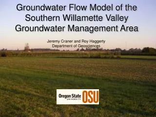
Southern Willamette Valley groundwater flow model.

E N D
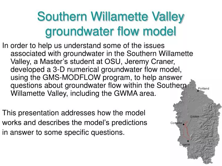
Southern Willamette Valley groundwater flow model In order to help us understand some of the issues associated with groundwater in the Southern Willamette Valley, a Master’s student at OSU, Jeremy Craner, developed a 3-D numerical groundwater flow model, using the GMS-MODFLOW program, to help answer questions about groundwater flow within the Southern Willamette Valley, including the GWMA area. This presentation addresses how the model works and describes the model’s predictions in answer to some specific questions.
What can a model do? A model is a representation of real-world relationships, which can be used to make predictions about what will happen in the real world. Models can be used to help us understand complex problems, such as groundwater flow in the Southern Willamette Valley. Because we do not completely understand this problem, we must simplify it and make some assumptions about relationships between components of the problem. What can a model NOT do? Models cannot answer every question we might have. They can rarely incorporate every aspect of a problem. They may not provide completely accurate answers. In short, models can only make an approximation based on the information we give them. • Some of the assumptions made in this particular model, as well as some of the input, or actual data put into the model, are described in the following two slides
BOUNDARY CONDITIONS Generalized Head Boundary South Santiam River Mary’s River Calapooia River Willamette River NO FLOW Boundary Muddy Creek Long Tom River McKenzie River NO FLOW Boundary Scale 5 miles Generalized Head Boundary Generalized Head Boundary Some assumptions made in this model • Groundwater only flows into or out of the model: • At the generalized head boundaries shown at right. • In evapotranspiration, irrigation and recharge • The model does not have seasons. • Rainfall is averaged over the entire area. • Nitrate travels advectively – that is, it travels with water particles, at the same speed and in the same direction as water particles. • Groundwater flow is modeled in square areas which are 500 feet on a side – or roughly 6 acres in area.
A’ A Model Input • Irrigation water usage information from Conlon et al., 2005 • Maximum potential evapotranspiration = 45 in/yr • Precipitation = 28 in/yr – data was collected during a dry year! • Recharge = 7.6 in/yr • Geologic layers as shown below: As new data is collected, and we better understand the relationships described in the model, we can improve, or refine, the model.
Questions for the model The MODFLOW groundwater flow model can be used to determine groundwater flow direction, groundwater velocities, and be used to help solve problems. We can use the model to help us to answer a wide variety of questions, though the answers depend on the assumptions we make in constructing the model. Here we ask three questions about groundwater in the Southern Willamette Valley. • How long does nitrate take to move from one point to another within the valley? • Specifically, in what direction and how fast do we expect nitrate to travel in the Bottom Loop Road area of Coburg? • What are the effects of groundwater pumping on local groundwater and surface water?
Scale 5 miles What is the travel time of nitrate in the groundwater? Simulated particles were tracked from their release at the water table to the time at which they reached either a model boundary or a river. The map shows the time that the particle took, or its travel time, at the particle’s starting location. This problem was modeled in both the middle and lower sedimentary hydrogeologic units. Years Years Middle sedimentary hydrogeolgic unit Lower sedimentary hydrogeolgic unit Mean travel time = 29 years Mean travel time = 100 years WHAT DOES THIS MEAN?
Implications of travel time maps • Travel time can be helpful in determining: • when to sample groundwater for nitrate • how to manage land over old vs. young groundwater • For example, determining an appropriate well depth to minimize nitrate contamination may depend on the age of the groundwater under your property • approximately how long it will take for changes in water-quality related practices to be have a measurable effect • These maps suggest that if we start implementing such practices today, it could be decades before groundwater nitrate concentrations are reduced
How fast and where does nitrate in the groundwater around Coburg travel? Particles representing nitrate were released in the model at the block dots shown here. The blue arrows represent the model’s prediction of particles’ locations after 1000 days, if they had not already reached the Willamette River. W E This cross section suggests that particles would travel just below the water table, in the middle sedimentary hydrogeologic unit. Middle sedimentary hydrogeologic unit Lower sedimentary hydrogeologic unit WHAT DOES THIS MEAN? x20 vertical exaggeration
Implications of modeled groundwater flow direction in Coburg area • Are you up-gradient from your neighbor? • The map output from the model shows that groundwater flows roughly from East to West, towards the Willamette River, along the gradient shown by the yellow arrows • Thus what you put into the groundwater at your property may be found in the well of someone down-gradient, or towards the Willamette. • Also, contaminant migration direction and travel time give local officials estimates of where to monitor groundwater and the clean-up time of groundwater if current management practices change.
What are the effects of wells on groundwater and surface water? A simulated well, pumping 750 gallons/minute, was placed West of the Willamette and Harrisburg. The simulation was run twice, pumping at two different depths. well locations Middle Sedimentary Hydrogeologic Unit (MSHU) MSHU well LSHU The model predicts that a well pumping from the MSHU would draw from a narrow area and that travel times would be relatively fast. The water would travel from the MSHU, down to the LSHU, and back to the well in the MSHU. Blue arrows show water particle location every 100 days. Lower Sedimentary Hydrogeologic Unit (LSHU) MSHU LSHU well The model predicts that a well pumping from the LSHU would draw from a wide area, and that water would pass beneath the Willamette River. The pumped water would originate at the water table, travel to the LSHU, and then move nearly horizontally to the pumping well. Blue arrows show water particle location every 1000 days. WHAT DOES THIS MEAN?
Implications of well simulations • This simulation can aid in determining well placement, well capture zones, and effects of pumping on the nearby Willamette River. • For example, wells drilled into the Lower Sedimentary Hydrogeologic Unit (LSHU) draw from a wider area and thus may have a greater chance for contamination, depending on whether that area intersects with any major areas of contamination
Water Quality Conservation Practices There are a variety of practices which we may use to decrease the amount of nitrogen we add to groundwater. These may include: • timing of fertilizer application • timing of irrigation quantities and rates • appropriate technologies and maintenance of home septic systems and wells To learn more about such recommendations, see the Southern Willamette Valley Groundwater Management Area Action Plan.
credits • The GMS-MODFLOW model was developed by Jeremy Craner as part of an M.S. thesis at Oregon State University. • The presentation was developed by Laila Parker at Oregon State University.