Download
1 / 91
910 likes | 1.08k Views
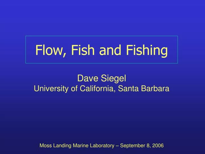
Flow, Fish and Fishing. Dave Siegel University of California, Santa Barbara Moss Landing Marine Laboratory – September 8, 2006. U.S. West Coast Rockfish. Source: Pacific Fisheries Management Council, 2001. I was a victim of public service.

E N D
Flow, Fish and Fishing Dave Siegel University of California, Santa Barbara Moss Landing Marine Laboratory – September 8, 2006
U.S. West Coast Rockfish Source: Pacific Fisheries Management Council, 2001
I was a victim of public service... • Served on Science Panel for the Channel Islands Marine Reserve Working Group • Build a marine protected area to achieve both conservation & fishery objectives • protectbiodiversity • maintain fishery yields & incomes
Approved Oct. 24, 2002 State waters are implemented
MPA’s increase local stocks • Leads to spillover of fish for harvest Spillover MPA Distance -> How a MPA might work Fish(x) Key: Spatial Management of a Fishery
Who are we talking about?? • Harvested species with limited home ranges • Rockfish, kelp bass, urchin, … • Not tuna, sardine, whales, ...
So, How a MPA might work?? • MPA’s allow adults grow to maturity (especially for sedentary fish & inverts) • Elimination of harvest enables more “natural” communities & food webs to exist • Fecundity for many fish increase with age • Fishery benefits if progeny disperse broadly or adults “spill out” of the MPA
Conservation vs. Fisheries Conservation Goal Value Fishery Goal Fractional Set Aside
Will a MPA Work for Conservation? • Yes, the “field of dreams” works • If you build an MPA, fish will come... • Lots of empirical evidence • Larger, more productive adults, more robust, “natural” food webs, etc. • Biodiversity goals will be satisfied
MPA’s Work Within Their Borders From Halpern [2002]
Will a MPA Work for Fisheries? • A few case studies show nearby fisheries benefiting from a MPA • BUT, what about the general case? • How do we predict spillover from a MPA & its role on nearby fisheries? • Theory is not well advanced...
A Typical Life Cycle • Larvae are released to develop in plankton • They disperse in the currents • A select few settle on suitable habitat • Even fewer recruit to adults • The cycle repeats (if they’re lucky) KEY ELEMENT => Larval Transport
Fishery Models for MPA’s Next generation stocks = survivors - harvest + new recruits SURVIVORS are those naturally surviving adults HARVEST are those extracted NEW RECRUITS are a function of fecundity of the survivors, larval dispersal & mortality, settlement & recruitment to adult stages
Dispersal Kernel Mathematically...
Dispersal Kernels • A dispersal kernel defines probability of successful larval settling as function of distance from a site • Units of [settlers / km / total settlers] K(x) X=0 Distance alongshore [km]
Objectives of this talk • Characterize the larval dispersal Address the time/space scales of “connectivity” Understand competing roles of biology & physics • Develop bio-physical models of larval transport • Markov chain modeling of larval dispersal • Regional Ocean Modeling System (ROMS) • Release & advect larvae using simulated flows • Assess where they settle -> connectivity matrices
Dispersal Scales for Marine Organisms Kinlan & Gaines [2003], Ecology
Dispersal & Time in Plankton Genetic Dispersal Scale (km) The longer the development time, the further the mean dispersal Pelagic Larval Duration (days) • Siegel et al. [2003; Marine Ecology Progress Series 260: 83-96]
Modeling Larval Dispersal • Larvae are advected & dispersed by coastal circulations as they develop competency to settle in suitable habitat • Important elements for modeling dispersal • Pelagic larval duration (PLD) What is the development time window for the organism? • Ocean circulation (mean & fluctuating currents) • Larval behavior (depth strata that larvae prefer)
Coastal flows are highly variable... HF Radar Surface Currents - Libe Washburn [UCSB]
Lagrangian paths are too.. All drifter tracks from GOIN - Data from CCS/SIO
Where do drifters settle? Location of “settlement” of GOIN drifters - Winant et al. [1999]
Modeling of Larval Transport - 1 • Model trajectories of many individual larvae • Correlated random walk - Markov chain • Use realistic ocean velocity statistics for surface flow • Homogeneous ocean with different values of U, su & tL • A “CODE-like” scenario following Davis [1981] • Requires larval development time scenario - biology • Ensemble averaging provides dispersal kernel Siegel, Kinlan, Gaylord & Gaines [2003; MEPS]
Example Trajectories PLD = 0 to 5 days PLD = 6 to 8 weeks U = 5 cm/s & su = 15 cm/s
Estimate of Dispersion Kernels PLD = 0 to 5 days PLD = 6 to 8 weeks • K(x) defines along shore settling probability distribution • Trajectories are summed to determine K(x)
Kernel Modeling Results A Gaussian form for K(x) seemed to hold for nearly all flow/settling protocols Mean currents regulate offset (xd) RMS flow drives spread (sd) & amplitude (Ko)
Kernel Modeling Scaling Ko = f(1/(PLD su)) xd = f(PLD U) “Offset” “Amplitude” Dd = dispersion scale “Spread” sd = f(PLD su2)
A Model Validation? Modeled Dispersion Scale, Dd (km) Genetic Dispersion Scale (km)
Another Model Validation?? Scripps/MMS Drifter Beachings o = release site & + = beaching Data from Ed Dever (OSU)
Drifter Model Validation?? PLD = 2 d U = 15 cm/s su = 15 cm/s PLD = 7 d U = 5 cm/s su = 15 cm/s
Markov Chain Results • Dispersal kernels can be estimated using simple particle dispersion theory • K(x)’s are to O(1) Gaussian & are parameterized using simple flow & life history information • Dispersal modeling is roughly consistent with genetic & beached drifter estimates • Time scales are important… but ignored here
Invert Settlement Time Series – Ellwood, CA PISCO / SBC-LTER [UCSB]
Interpreting Settlement Time Series • Stochastic, quasi-random time series • No correlation in settling among species • Relatively few settlement events for each species • Events are short (typically £ 2 days)
Time, continued... • Annual recruitment may be a small sampling of a dispersal kernel (N = 10?, or less!!) • (300 releases / year) * (10% survival) / (3 day tL) • Example for N= 100 -> • Implies that connectivity is stochastic & intermittent N=5000
A Stirred, Not Mixed Ocean! • Stochasticity in larval settlement is created from sampling only a few trajectories • Larval transport occurs in a stirred, not mixed ocean • Need to model the correlations in the flow to understand time / space scales of larval transport • To do this we use a coastal circulation model
Modeling of Larval Transport - 2 • Advect “larvae” using an ocean circulation model • Time dependent, 3D, quasi-realistic circulations • Regional Ocean Modeling System (ROMS) • Model summer-time conditions offshore of Pt Sur (CalCOFI line 70 – maximum upwelling conditions) • Uniform domain in the alongshore direction • Forcings based on observations Mitarai et al. in press, Journal of Marine Systems Siegel et al. in review, PNAS
Numerical Setting • Unstructured in alongshore direction (periodic BC) • Stochastic wind forcing at surface (stats from buoys) • Alongshore pressure gradient as a body force • Free slip inshore BC & open BC offshore 2-km horizontal resolution 20 vertical levels
Simulation field (mean over 180 days) CalCOFI data (July, Line #70) Model Validation Shows good agreement with CalCOFI mean
Model Validation Time scale Length scale Diffusivity Simulation data 2.7/2.9 d 29/31 km 4.0/4.3 x107 cm2/s Surface drifter data (Swenson & Niiler) 2.9/3.5 d 32/38 km 4.3/4.5 x107 cm2/s (along/cross shore) • Good agreement with surface drifter observations • Model disperses particles appropriately
Adding Larvae… • Pattern after rocky reef fish, BUT we want large number of successful settlement events • Large, uniform nearshore habitat (< 20 km) • Larvae are released daily for 90 days every 2 km • Settlement occurs for larvae aged 20 to 40 days • Biotic larval mortality is not considered • Source-destination relationship are calculated -> Assumptions lead to large settlement rates
Connectivity is Heterogeneous Connectivity diagrams show connection strength & locations of “hot spots” Settlement is patchy Peak is ~120 km upstream Self settlement happens Settlement is heterogeneous in an unstructured domain Source Location (km) Self settlement Destination Location (km)
Connectivity is Not Diffusive Source Location (km) Self settlement simulated diffusive Destination Location (km)
Connectivity is Intermittent 4 different realizations -> 4 different connectivity patterns
Connectivity Can Differ for Differing Life Histories Same flow Different PLD’s Different patterns caused by life history diff’s for the same flow Source Location (km) 20-40 d 5-10 d Destination Location (km)
Connectivity Can Differ for Differing Larval Behaviors Same flow Enable simple vertical migration Different patterns arise due to larval behavior diff’s Source Location (km) surface migration Destination Location (km)
Connectivity is Still Stochastic for a Sinuous Coastline Same flow but a sinuous coastline Patterned after CA coast “Hot spots” do NOT follow coastline features surface migration
Summary of Modeling Results • Larval connectivity patterns are heterogeneous & intermittent & NOT diffusive (even for a uniform region!!) • Life history can alter connectivity patterns (for same flow) • Arriving larvae come in “packets” (scaling theory developed) • Self-seeding & distant transport occur as rare, discrete settlement events (influencing alee effects) • Present case optimizes successful settlement Nearly any change will make stochasticity worse!!