Download
1 / 66
660 likes | 928 Views
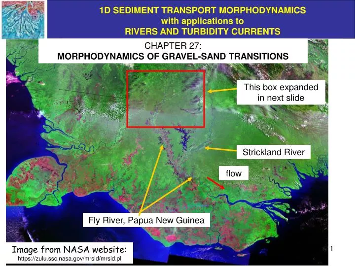
CHAPTER 27: MORPHODYNAMICS OF GRAVEL-SAND TRANSITIONS. This box expanded in next slide. Strickland River. flow. Fly River, Papua New Guinea. Image from NASA website: https://zulu.ssc.nasa.gov/mrsid/mrsid.pl. THE BOX IS EXPANDED IN THE NEXT SLIDE TO SHOW A GRAVEL-SAND TRANSITION. Ok Tedi.

E N D
CHAPTER 27: MORPHODYNAMICS OF GRAVEL-SAND TRANSITIONS This box expanded in next slide Strickland River flow Fly River, Papua New Guinea Image from NASA website: https://zulu.ssc.nasa.gov/mrsid/mrsid.pl
THE BOX IS EXPANDED IN THE NEXT SLIDE TO SHOW A GRAVEL-SAND TRANSITION Ok Tedi flow flow Fly River Image from NASA website: https://zulu.ssc.nasa.gov/mrsid/mrsid.pl
GRAVEL-SAND TRANSITION ON THE OK TEDI, PAPUA NEW GUINEA flow Wandering gravel-bed river Gravel-sand transition Meandering sand-bed river flow Image from NASA website: https://zulu.ssc.nasa.gov/mrsid/mrsid.pl
GRAVEL-SAND TRANSITION ON THE BENI RIVER, BOLIVIA Image courtesy R. Aalto: see Aalto (2002) flow Foredeep: zone of tectonic susidence Gravel-sand transition Andes mountains: zone of high tectonic uplift flow
GRAVEL-SAND TRANSITION ON THE BENI RIVER, BOLIVIA contd. Note the discontinuity in grain size at the gravel-sand transition. Image courtesy R. Aalto: see Aalto (2002) flow
GRAVEL-SAND TRANSITION ON THE BENI RIVER, BOLIVIA contd. Note the discontinuity in slope at the gravel-sand transition. Image courtesy R. Aalto: see Aalto (2002) flow
GRAVEL-SAND TRANSITION: KINU RIVER, JAPAN Long profile showing downstream fining and gravel-sand transition in the Kinu River, Japan (Yatsu, 1955) Both the gravel-bed and sand-bed reaches have upward-concave profiles, and show downstream fining. Note the sharp breaks in slope and grain size! Sambrook-Smith and Ferguson (1995) have documented many relatively sharp gravel-sand transitions in rivers around the world.
SHARP GRAVEL-SAND TRANSITIONS ARE LIKELY ASSOCIATED WITH A RELATIVE PAUCITY OF MATERIAL IN THE RANGE 2-8 MM IN MANY RIVERS This paucity was illustrated in Chapters 2 and 3. It is common, but by no means universal. From Chapter 3 From Chapter 2
THE SIMPLEST WAY TO MODEL LONG PROFILES WITH GRAVEL-SAND TRANSITIONS IS TO CONSIDER A TWO-GRAIN SYSTEM The bed material of the gravel-bed reach is characterized with a single size Dg. The bed material of the sand-bed reach is characterized with a single size Ds. The position of the gravel-sand transition is x = sgs. It is assumed that the sand is transported through the gravel-bed reach as wash load. L = reach length g = elevation of gravel bed s = elevation of sand bed
SIMPLIFICATIONS OF THE PRESENT MODEL • The model of this chapter focuses on gravel-sand transitions in subsiding basins, and in rivers-floodplain complexes subject to sea-level rise. The following simplifications are introduced. • The gravel is characterized with a single grain size Dg, and the sand is characterized with a single grain size Ds. Grain size mixtures of gravel and sand are not considered. • The total length of the gravel-bed reach plus the sand-bed reach = the constant value L. The position of the gravel-sand transition x = sgs(t) may change in time. • No allowance is made for delta progradation. • Abrasion of gravel to sand is neglected. • It is assumed that there are no significant tributaries along the entire reach from x = 0 to x = L, so that water discharge during floods is constant downstream. • Each reach (gravel-bed and sand-bed) is assumed to have a constant width. • None of these assumptions would be overly difficult to relax.
PARAMETERS AND EXNER EQUATIONS • x = downchannel spatial coordinate [L] • t = time [L] • g, s = bed elevation on gravel-bed, sand-bed reach [L] qg, qs = total volume gravel load, sand load per unit width [L2/T] pg, ps = bed porosity of gravel-bed, sand-bed reach [1] Ifg, Ifs = flood intermittency on gravel-bed, sand bed reach [1] g, s = channel sinuosity on gravel-bed, sand-bed reach [1] sg, ms = volume fraction sand deposited per unit gravel, volume fraction mud deposited per unit sand in channel-floodplain complex [1] rBg, rBs = ratio of channel width Bc to depositional width Bd (basin or floodplain width) in gravel-bed, sand-bed reach (Bd,grav/Bc,grav or Bd,sand/Bc,sand) = subsidence rate [L/T] Based on the formulation of Chapter 25, the conservation relations for gravel and sand on the gravel-bed reach are The conservation relation for sand on the sand-bed reach is
CONTINUITY CONDITION AT THE GRAVEL-SAND TRANSITION Let ssg(t) denote the position of the gravel-sand transition, and Sggs and Ssgs denote the gravel bed slope and sand bed slope, respectively, at the gravel-sand transition, so that
CONTINUITY CONDITION AT THE GRAVEL-SAND TRANSITION contd. In analogy to the treatment of bedrock-alluvial transitions in Chapter 16, bed elevation continuity at the gravel-sand transition is expressed in the following form: Taking the derivate of both sides of the above equation with respect to t and rearranging with the definitions of Sggs and Ssgs of the previous slide, it is found that where = dssg/dt denotes the migration speed of the gravel-sand transition. Since gravel is harder to move than sand, it can be expected that Sggs > Ssgs. Now suppose that near the gravel-sand transition the sand-bed reach is aggrading faster than the gravel-bed reach, i.e. s/t > g/t. According to the above equation, then, and the gravel-sand transition migrates upstream.
THE LOCATION OF THE GRAVEL-SAND TRANSITION CAN STABILIZE! Consider a subsiding system that has reached a steady state, as described in Chapter 26: In such a case the continuity condition yields the result i.e. an arrested gravel-sand transition (Parker and Cui, 1998; Cui and Parker, 1998). If such a steady-state position exists, the system will naturally evolve toward it. Sea level rise at a constant rate can also lead to an arrested gravel front when the following condition is satisfied:
MAXIMUM REACH LENGTH FOR STEADY STATE SYSTEM In the case of a steady-state system entering a basin subsiding at constant rate with constant base level, the governing equations for the gravel-bed reach reduce to and the governing equation for the sand-bed reach reduces to The corresponding forms for the case of a constant rate of base level (sea level) rise in the absence of subsidence are These forms are closely allied to the steady-state forms developed in Chapter 26. Gravel-bed reach Sand-bed reach
MAXIMUM REACH LENGTH FOR STEADY STATE SYSTEM contd. In general, then, the steady-state equations can be written as where vv = for the case of constant subsidence without base level rise and vv = for the case of base level rise at a constant rate without subsidence. Over the gravel-bed reach, the top two equations integrate to where qg,feed and qs,feed denote the feed rates of sand and gravel (volume feed rate per unit width) at x = 0. Gravel-bed reach Sand-bed reach Gravel and sand fill the accommodation space of the gravel-bed reach created by subsidence or sea level rise.
MAXIMUM REACH LENGTH FOR STEADY STATE SYSTEM contd. The gravel transport rate drops to zero (qg = 0) at the steady-state position of the gravel-sand transition x = ssg,ss given by the relation The sand transport rate qs at the point where the gravel runs out is Note that in order for sand to be available for transport beyond x = Lgrav,max the following condition must be satisfied: The relation for the sand-bed reach (second equation of previous slide) then integrate to give
MAXIMUM REACH LENGTH FOR STEADY STATE SYSTEM contd. The sand transport rate drops to zero (qs = 0) at x = Lmax, given by the relation or thus If the reach length is longer than Lmax it is not possible to reach a steady state which maintains a specified base level at the downstream end of the reach. This is because there is not enough sediment (gravel and sand) available to fill the accomodation space created by subsidence or sea level rise. The result is the formation of an embayment (drowned river valley) at the downstream end.
REDUCTION OF THE CONTINUITY CONDITION TO A RELATION FOR THE MIGRATION SPEED OF THE GRAVEL-SAND TRANSITION Returning to the non-steady-state problem, the continuity condition reduces with the forms for Exner of Slide 11, i.e. to yield the following equation for the migration speed of the gravel-sand transition:
TRANSFORMATION TO MOVING BOUNDARY COORDINATES The gravel-sand transition is free to move about in time. It thus constitutes a moving boundary problem. Moving boundary analysis was developed in the context of a migrating bedrock-alluvial transition in Chapter 16. Here it is adapted for the case of a gravel-sand transition. Moving boundary coordinates for the gravel-bed and sand-bed reaches can be defined as: Note that on the gravel-bed reach, and on the sand-bed reach. The Exner equation for gravel conservation on the gravel-bed reach of the previous slide transforms to:
TRANSFORMATION TO MOVING BOUNDARY COORDINATES contd. The Exner equation for the conservation of sand on the gravel-bed reach, given in Slide 11, transforms to: The Exner equation for the conservation of sand on the sand-bed reach, given in Slide 15, transforms to: The continuity condition of Slide 12 describing the migration speed of the gravel-sand transition transforms to:
SPATIAL DISCRETIZATION The spatial discretization involves MG gravel-bed intervals followed by MS sand-bed intervals, bounded by MG + MS + 1 nodes. The dimensionless spatial steps for the gravel-bed and sand-bed reaches are given as The node i = MG + MS + 1 defines the downstream end of the reach, i.e. x = L. The node i = MG + 1 defines the gravel-sand transition, i.e. x = sgs. Gravel and sand are fed in at a ghost node one step upstream of node i = 1.
CALCULATION OF FLOW A backwater formulation is used to compute the flow (which is assumed to be barely confined to the channel). The friction coefficients on the gravel-bed and sand-bed reaches, denoted correspondingly as Cfg and Cfs, are assumed to be specified constants. In accordance with Chapter 5, then, the backwater formulation for the gravel-bed reach is where Hgrav denotes flow depth on the gravel-bed reach, qw denotes the water discharge per unit width (during floods) and Sg denotes bed slope on the gravel-bed reach, and the corresponding formulation for the sand-bed reach is where Ss denotes the slope and Hsand denotes the flow depth on the sand-bed reach.
CALCULATION OF FLOW contd. Transforming the relations of the previous page to moving boundary coordinates results in the forms
CALCULATION OF FLOW contd. The boundary condition on the backwater formulation is specified at x = L, where downstream water surface elevation d is specified. Here may be a specified constant do , or it may change in time at some constant rate . Thus in general or In addition, a continuity condition must be satisfied at the gravel-sand transition;
CALCULATION OF FLOW contd. At any given time, the backwater curve above the bed at that time can then be solved numerically by implementing the formulation of Chapter 20 adapted to the present problem. That is, for the sand-bed reach
CALCULATION OF FLOW contd. The corresponding formulation for the gravel-bed reach is
CALCULATION OF SHIELDS NUMBERS The submerged specific gravity R = s/ - 1 is assumed to be the same for the gravel as it is for the sand. Recall from Chapters 5 and 20 that boundary shear stress b is given as where H denotes flow depth, and that the Shields number * is given as where D is an appropriate grain size. Let U = qw/H. The Shields number sand,i* at the ith node of the sand-bed reach is thus given as and the corresponding value grav,i* for the ith node of the gravel-bed reach is given as
CALCULATION OF SEDIMENT TRANSPORT In the present implementation the gravel transport on the gravel-bed reach is calculated using the Parker (1979) approximation of the Einstein (1950) relation introduced in Chapter 7; where qg denotes the volume gravel transport per unit width and the subscript “i” denotes the ith node, The sand transport on the sand-bed reach is calculated using the Engelund-Hansen (1967) formulation introduced in Chapter 12; where qs denotes the volume sand transport per unit width and the subscript “i” denotes the ith node,
CALCULATION OF BED EVOLUTION OF GRAVEL-BED REACH The implementation of Exner on the gravel-bed reach is as follows: where qg,feed denotes the volume feed rate per unit width of gravel at x = 0,
CALCULATION OF CAPTURE OF SAND IN THE GRAVEL-BED REACH The model is designed so that washload (e.g. sand for a gravel-bed stream) can be captured as the gravel-bed channel aggrades over its depositional width. This results in a downstream decrease in qs over the gravel-bed reach, even though sand is traveling as wash load. The decrease is calculated by discretizing the following relation from Slide 21: so yielding where qs,feed denotes the volume feed rate per unit width of sand at x = 0.
CALCULATION OF BED EVOLUTION OF SAND-BED REACH The implementation of Exner on the sand-bed reach is as follows:
CALCULATION OF MIGRATION OF GRAVEL-SAND TRANSITION The migration speed of the gravel-sand transition is given as: This relation translates to the following moving-boundary form: where The new position of the gravel-sand transition is thus given as
INTRODUCTION TO RTe-bookGravelSandTransition.xls, A CALCULATOR FOR THE EVOLUTION OF THE LONG PROFILE OF A RIVER WITH A GRAVEL-SAND TRANSITION THAT IS FREE TO MIGRATE The analysis of the previous slides is implemented in the workbook RTe-bookGravelSandTransition.xls. The code utilizes a large number of input parameters in worksheet “InData”, as enumerated below and on the next slide Qbf bankfull discharge: same for gravel- and sand-bed reach [L3/T] Ifg flood intermittency for gravel-bed reach [1] Ifs flood intermittency for sand-bed reach [1] Qgrav,feed volume feed rate of gravel at x = 0 (qg,feed = Qgrav,feed/Bc,grav) [L3/T] Qsand,feed volume feed rate of sand at x = 0 (qs,feed = Qsand,feed/Bc,sand) [L3/T] Bc,grav bankfull width of gravel-bed stream [L] Bc,sand bankfull width of sand-bed stream [L] Bd,grav depositional width of gravel-bed reach (rBg = Bd,grav/Bc,grav) [L] Bd,sand depositional width of sand-bed reach (rBs = Bd,sand/Bc,sand) [L] g sinuosity of gravel-bed reach [1] s sinuosity of sand-bed reach [1] sg volume fraction of sand deposited per unit gravel in gravel-bed reach [1] ms volume fraction of mud deposited per unit sand in sand-bed reach [1] Dg characteristic size of gravel [L] Ds characteristic size of sand [L]
INTRODUCTION TO RTe-bookGravelSandTransition.xls contd. More input parameters specified in worksheet “InData” of RTe-bookAgDegNormalGravMixSubPW.xls are defined below. Czg Chezy resistance coefficient of gravel-bed reach (Cfg = Czg-2) [1] Czs Chezy resistance coefficient of sand-bed reach (Cfs = Czs-2) [1] L Reach length [L] sgsI Initial value of distance sgs to gravel-sand transition [L] SgI Initial slope of gravel-bed reach [1] SsI Initial slope of sand-bed reach [1] Subsidence rate [L/T] do Initial value of sea level elevation [L] rate of sea level rise [L/T] Yearstart Year in which sea level rise starts [T] Yearstop Year in which sea level rise stops [T] t Time step [T] MG Number of gravel intervals MS Number of sand intervals Mtoprint Number of time steps to printout Mprint Number of printouts The following parameters are specified in worksheet “AuxiliaryData”: porosity of deposit on gravel-bed reach pg, porosity of deposit on sand-bed reach ps and sediment submerged specific gravity R (assumed to be the same for sand and gravel).
NOTES AND CAVEATS • The code locates the gravel-sand transition at a point determined by the continuity condition. At this point the gravel transport rate is only a small fraction of the feed value, but it is not precisely zero. In rivers, the small residual gravel load at gravel-sand transitions is either buried or consists of grains that easily break down to sand. In the code, the residual gravel load at the gravel-sand transition is added to the sand load. • In the case of sea level rise at constant rate , rise can be commenced and halted at specified times Yearstart and Yearstop in worksheet “InData”. • The reach length L should be chosen to be less than the maximum value Lmax, in order to ensure that there is enough sediment supply to fill the accomodation space created by subsidence or sea level rise. Guidance in this regard is provided in Cell C41 of worksheet “InData”. • The initial downstream bed elevation is taken to be zero. As a result, the initial downstream water surface elevation do also equals the initial downstream depth. In order to ensure subcritical flow (and thus keep the calculation from crashing), do must be exceed the critical flow depth Hc = [(Qbf/Bc,sand)2/g]-1/3. Guidance is provided in Cell C44 of worksheet “InData”. • Depending on the input values, there may be no steady-state solution allowing a gravel-sand transition to equilibrate at a position between 0 and L. For example, if = 0 and = 0, the only steady-state solution is one for which the sand is all driven into the sea. In such cases, the code will fail. (It would be an easy job to modify the code to handle such cases, but it has not been done). The code can be run, however, to a time at which the gravel-sand • transition is nearly driven out of the domain of interest. Examples appear • in succeeding slides.
EVOLUTION OF RIVER PROFILES WITH MIGRATING GRAVEL-SAND TRANSITIONS: CASE OF SEA LEVEL RISE (WITH VANISHING SUBSIDENCE) A parametric study is presented with rates of sea level rise varying from 0 to 14 mm/year. Input data for a base case ( = 6 mm/year) are given to the left and below.
d/dt = 0 mm/year SEA LEVEL RISE OF 6 MM/YEAR FOR 6000 YEARS Gravel-sand transition
d/dt = 0 mm/year SEA LEVEL RISE OF 6 MM/YEAR FOR 6000 YEARS Position of gravel-sand transition migrates downstream and stabilizes as river aggrades.
d/dt = 0 mm/year SEA LEVEL RISE OF 6 MM/YEAR FOR 6000 YEARS The high slope near the gravel-sand transition is an artifact of the calculation and should be ignored: see next slide. Gravel-bed Slope break at gravel-sand transition at steady state Sand-bed
d/dt = 0 mm/year REASON FOR THE SPURIOUSLY HIGH GRAVEL-BED SLOPE NEAR THE GRAVEL-SAND TRANSITION In a backwater formulation, the actual continuity condition is not the one given in Slide 13 in terms of bed elevation but rather one expressed in terms of water surface elevation: Since = + H, this leads to the form The extra terms would likely remove the spurious slope, but would otherwise not change the analysis much.
d/dt = 0 mm/year SEA LEVEL RISE OF 6 MM/YEAR FOR 6000 YEARS Sand load does not drop to zero even at steady state Sand Gravel load drops nearly to zero at steady-state gravel-sand transition Gravel
SEA LEVEL RISE OF 6 MM/YEAR FOR 6000 YEARS The gravel-sand transition migrates downstream nearly to its steady state position within 2000 years.
SEA LEVEL RISE OF 0 MM/YEAR FOR 6000 YEARS The model eventually fails shortly after 2160 years as the gravel-sand transition migrates downstream out of the domain. This is to be expected for a vanishing sea level rise.
SEA LEVEL RISE OF 2 MM/YEAR FOR 6000 YEARS Again the gravel-sand transition migrates downstream out of the domain, this time shortly after 3780 years. The rate of sea level rise is still not sufficient to stabilize the gravel-sand transition within the domain.
SEA LEVEL RISE OF 3 MM/YEAR FOR 6000 YEARS Gravel-sand transition location does not stabilize by 6000 years, but neither does it migrate downstream out of the domain.
SEA LEVEL RISE OF 4 MM/YEAR FOR 6000 YEARS Gravel-sand transition migrates downstream and starts to stabilize by 6000 years.
SEA LEVEL RISE OF 6 MM/YEAR FOR 6000 YEARS Gravel-sand transition migrates downstream modestly and stabilizes by 6000 years.
SEA LEVEL RISE OF 8 MM/YEAR FOR 6000 YEARS Gravel-sand transition migrates slightly upstream and stabilizes by 6000 years.
SEA LEVEL RISE OF 10 MM/YEAR FOR 6000 YEARS Gravel-sand transition migrates supstantially upstream and nearly stabilizes by 6000 years.