Download
1 / 21
240 likes | 435 Views
The History of Fire Modelling with comments on How Savannas are Different. Bob Scholes CSIR Environmentek Bscholes@csir.co.za. A taxonomy of fire models. F, E. Byram’s conceptual ‘model’. L. t1. t2. I = F*H*ROS. I=fireline intensity (kW/m/s) F=fuel load (kg/m 2 )

E N D
The History of Fire Modellingwith comments onHow Savannas are Different Bob Scholes CSIR Environmentek Bscholes@csir.co.za
F, E Byram’s conceptual ‘model’ L t1 t2 I = F*H*ROS I=fireline intensity (kW/m/s) F=fuel load (kg/m2) H=energy content of fuel (~18 MJ/kg) ROS=rate of spread = L/(t2-t1) = m/s Byram, GM 1959 Combustion of forest fuels. In Davis, KP (ed) Forest fire control and use. McGraw-Hill, NY 61-89
Empirical behavior models • Predict RoS and/or Intensity on the basis of fuel load and meteorology • McArthur 1966 • CSIRO grass fire spread nomogram (humidity,temperature, degree curing, wind speed, slope) • Trollope and Potgieter (1985) • (fuel load, humidity, wind speed, temperature) Used for risk prediction and fire control McArthur, AG 1966 Weather and grassland fire behavior. Dept Forests, Canberra Trollope, WSW and Potgieter ALF 1985 Fire behavior in the Kruger National Park. J Grassld Soc Sthn Af 3:148-52
Intensity and flame length I = 401 H 1.95 I~400 H2 or H ~ sqrt (I)/20 • Simple way to estimate intensity in the field • Fuel available • Easy way to predict tree mortality • if Htree<Hflame then die Hflame Van Wilgen (1986) SAJBot 52,384-385
Rothermel’s semi-mechanistic fire behavior model • Concept of fuel components • Based on time to reach moisture equilibrium with the air • Eg ‘1 hour fuels’ such as fine dry grass, 10 hr twigs etc • Concept of ‘fuel packing’ • Arrangement of fuels in 3-D space • Relatively complex models with many parameters • Basis of most modern fire behavior models and some fire risk prediction systems Rothermel, RC 1972 A mathematical model for predicting fire spread in wildland fuels. USDA Forest Service Res Pap INT 115
Seiler & Crutzen emission model E = A*F*C*EF E = emission of a gas or particle (g) [g x 105] A = area burned (m2) [km2] ~ Total area/mean fire return time F = fuel load (g/m2) [t/ha] C = combustion completeness (gburned/gexposed) EF = emission factor (ggas/gfuel) [g/kg] Seiler,W & Crutzen, PJ 1980 Estimates of gross and net fluxes of carbon between The biosphere and the atmosphere from biomass burning Clim Change 2, 207-247 Crutzen, PJ and Andreae MO 1990 Biomass burning in the tropics: impact on atmospheric chemistry and biogeochemical cycles. Science 250: 1669-1678
Hao et al: spatial application • 5 x 5 grid over tropical Africa, Asia and America • Applied Seiler & Crutzen formula to each • Assumed one fuel load for all savannas (~5 t/ha) and • A high burned area fraction (~0.8) Hao WM, Liu MH & Crutzen PJ 1990 In Goldammer, PJ Fire in the Tropical Biota. Springer. Ecological Studies 84,440-462
Scholes et al: continuous fields • 0.5 x 0.5 degree grid over southern Africa • Crutzen formula, but fuel loads modelled from climate, vegetation and herbivory fields • 5 fuel categories: green & dry grass, litter, twigs, wood • Burned area from calibrated AVHRR • Emission factors from Ward relation Scholes RJ Kendall, J and Justice CO 1996 The quantity of biomass burned in southern Africa. JGR 101:23667-23676. Scholes, RJ, Ward, DE and Justice, CO 1996 Emissions of trace gases and aerosol Particles due to vegetation burning in southern hemisphere Africa.JGR 101:23677-23682
Classify or model continuously? • As nclasses or npoints2 the approaches become equivalent • Classification reduces computational effort without loss of accuracy if variation within the class is less than variation between • Known relationships between model inputs and some spatially continuous field (eg climate, RS), even if weak help to reduce uncertainty relative to using a class mean
Remote sensing approaches • Long history of fire detection and mapping from satellite (eg Setzer AW & MC Periera 1991 Ambio 20, 19-22) • True burned area needs high resolution, frequent overpass • Emission modeling using RS inputs (eg Kaufman et al 1990 JGR 95, 9927-9939) • Fuel load estimation (eg Tomppa et al 2002 RS&Env) • Fire completeness (Landmann in prep)
Burn completeness using satellite data Fires near Skukuza, South Africa. The black areas are scars from before the assessment period. The Shades of blue represent degrees of completeness as assessed using Landsat and Modis Landmann (in prep)
Hybrid approaches • Use remote sensing for burned area and to constrain plant production • Use FPAR, climate, soil and vegetation-driven models to generate fuel load • NPP = FPAR* *P/ET • Fueltypei = f(NPP, tree cover fraction,decay rate) • Context-sensitive completeness and emission-factors Eg Scholes (in prep)
Evolution of fire models Cellular automatons MacArthur 1966 Fire spread Intensity, ROS Ignition Remote sensing Combustion chemistry and physics ~1900 Byram 1959 Rothermal 1972 Burned area Fuel types Scholes 1996 Hybrid Emission factors Industrial Emission concepts Seiler &Crutzen 1980 Hao 1990
How are savannas different? • Frequent, low intensity, surface fires • Mixed tree and grass fuels • Grazing and human habitation • Fine fuel constrained, not ignition constrained
Frequent, low intensity fires • Not ‘stand transforming’ • Rapid regrowth of fuels means • High observation frequency needed for fire scar detection • Fuel load dynamic at sub-annual scale • At regional scale, annual fraction of area burned is much less variable than in forests • ~2 fold variation vs 10 fold • Fuelavailable<<aboveground phytomass+necromass
Mixed tree and grass fuels • Need 5 or more fuel categories to capture fuel dynamics and combustion characteristics • Dead grass, live grass, tree leaf litter, twig litter, large downed woody, [live tree leaf, dung] • Fuel composition varies spatially and temporally • f(tree cover, day of year, time since last fire) • Strong influence on emission factors and combustion completeness
Intensity F(fuel,H2O) Grass Litter Twig Wood ‘Bootstrapping’ completeness Cplot = a(1-exp(-b(I-I0)))
Grazing and human use • Carbon has alternate fates, each with emission consequences • Burned in wildfire; or in domestic fire; or eaten by herbivore or termite; or accumulates on land or in structures • In fertile savannas, up to 80% of aboveground NPP is grazed • (10-20% is more typical)
Fuel vs ignition constrained • In Africa, humans have been the dominant ignition agent for ~1 million years, in Australia for ~50 000 yr and in America for ~15 000 yr • Lightning only ~10% of ignitions • Burned area and emissions go down in fire seasons following a drought growing season, not up as in forests