Download

1 / 12
120 likes | 222 Views
Overview of query evaluation. Chpt 12. Overview of Query Optimization. Plan : Tree of R.A. ops, with choice of alg for each op. Each operator typically implemented using a `pull’ interface: when an operator is `pulled’ for the next output tuples, it `pulls’ on its inputs and computes them.

E N D
Overview of query evaluation Chpt 12
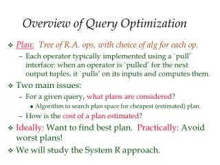
Overview of Query Optimization • Plan:Tree of R.A. ops, with choice of alg for each op. • Each operator typically implemented using a `pull’ interface: when an operator is `pulled’ for the next output tuples, it `pulls’ on its inputs and computes them. • Two main issues: • For a given query, what plans are considered? • Algorithm to search plan space for cheapest (estimated) plan. • How is the cost of a plan estimated? • Ideally: Want to find best plan. Practically: Avoid worst plans! • We will study the System R approach.
Highlights of System R Optimizer • Impact: • Most widely used currently; works well for < 10 joins. • Cost estimation: Approximate art at best. • Statistics, maintained in system catalogs, used to estimate cost of operations and result sizes. • Considers combination of CPU and I/O costs. • Plan Space: Too large, must be pruned. • Only the space of left-deep plans is considered. • Left-deep plans allow output of each operator to be pipelinedinto the next operator without storing it in a temporary relation. • Cartesian products avoided.
D D C C D B A C B A B A Left-deep join tree • Fundamental decision in System R: only left-deep join treesare considered. • As the number of joins increases, the number of alternative plans grows rapidly; we need to restrict the search space. • Left-deep trees allow us to generate all fully pipelined plans. • Intermediate results not written to temporary files. • Not all left-deep trees are fully pipelined
Schema for Examples Sailors (sid: integer, sname: string, rating: integer, age: real) Reserves (sid: integer, bid: integer, day: dates, rname: string) • Similar to old schema; rname added for variations. • Reserves: • Each tuple is 40 bytes long, 100 tuples per page, 1000 pages. • Sailors: • Each tuple is 50 bytes long, 80 tuples per page, 500 pages.
sname rating > 5 bid=100 sid=sid Sailors Reserves (On-the-fly) sname (On-the-fly) rating > 5 bid=100 (Simple Nested Loops) sid=sid Sailors Reserves RA Tree: Motivating Example SELECT S.sname FROM Reserves R, Sailors S WHERE R.sid=S.sid AND R.bid=100 AND S.rating>5 • Cost: 1000+500*1000 I/Os • By no means the worst plan! • Misses several opportunities: selections could have been `pushed’ earlier, no use is made of any available indexes, etc. • Goal of optimization: To find more efficient plans that compute the same answer. Plan:
(On-the-fly) sname (Sort-Merge Join) sid=sid (Scan; (Scan; write to write to rating > 5 bid=100 temp T2) temp T1) Reserves Sailors Alternative Plans 1 (No Indexes) • Main difference: push selects. • With 5 buffers, cost of plan: • Scan Reserves (1000) + write temp T1 (10 pages, if we have 100 boats, uniform distribution). • Scan Sailors (500) + write temp T2 (250 pages, if we have 10 ratings). • Sort T1 (2*2*10), sort T2 (2*4*250), merge (10+250) • Total: 4060 page I/Os. • If we used BNL join, join cost = 10+4*250, total cost = 2770. • If we `push’ projections, T1 has only sid, T2 only sid and sname: • T1 fits in 3 pages, cost of BNL drops to under 250 pages, total < 2000.
(On-the-fly) sname Alternative Plans 2With Indexes (On-the-fly) rating > 5 (Index Nested Loops, with pipelining ) sid=sid • With clustered index on bid of Reserves, we get 100,000/100 = 1000 tuples on 1000/100 = 10 pages. • INL with pipelining (outer is not materialized). (Use hash Sailors bid=100 index; do not write result to temp) Reserves • Projecting out unnecessary fields from outer doesn’t help. • Join column sid is a key for Sailors. • At most one matching tuple, unclustered index on sid OK. • Decision not to push rating>5 before the join is based on • availability of sid index on Sailors. • Cost: Selection of Reserves tuples (10 I/Os); for each, • must get matching Sailors tuple (1000*1.2); total 1210 I/Os.
Cost Estimation • For each plan considered, must estimate cost: • Must estimate costof each operation in plan tree. • Depends on input cardinalities. • We’ve already discussed how to estimate the cost of operations (sequential scan, index scan, joins, etc.) • Must estimate size of result for each operation in tree! • Use information about the input relations. • For selections and joins, assume independence of predicates. • We’ll discuss the System R cost estimation approach. • Very inexact, but works ok in practice. • More sophisticated techniques known now.
Statistics and Catalogs • Need information about the relations and indexes involved. Catalogstypically contain at least: • # tuples (NTuples) and # pages (NPages) for each relation. • # distinct key values (NKeys) and NPages for each index. • Index height, low/high key values (Low/High) for each tree index. • Catalogs updated periodically. • Updating whenever data changes is too expensive; lots of approximation anyway, so slight inconsistency ok. • More detailed information (e.g., histograms of the values in some field) are sometimes stored.
Size Estimation and Reduction Factors SELECT attribute list FROM relation list WHERE term1 AND ... ANDtermk • Consider a query block: • Maximum # tuples in result is the product of the cardinalities of relations in the FROM clause. • Reduction factor (RF) associated with eachtermreflects the impact of the term in reducing result size. Resultcardinality = Max # tuples * product of all RF’s. • Implicit assumption that terms are independent! • Term col=value has RF 1/NKeys(I), given index I on col • Term col1=col2 has RF 1/MAX(NKeys(I1), NKeys(I2)) • Term col>value has RF (High(I)-value)/(High(I)-Low(I))
Summary • Query optimization is an important task in a relational DBMS. • Must understand optimization in order to understand the performance impact of a given database design (relations, indexes) on a workload (set of queries). • Two parts to optimizing a query: • Consider a set of alternative plans. • Must prune search space; typically, left-deep plans only. • Must estimate cost of each plan that is considered. • Must estimate size of result and cost for each plan node. • Key issues: Statistics, indexes, operator implementations.