Download
1 / 51
510 likes | 652 Views
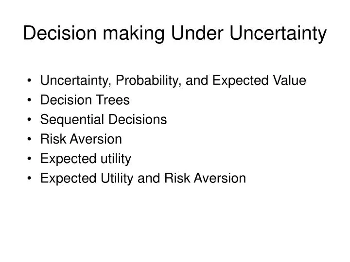
Decision making Under Uncertainty. Uncertainty, Probability, and Expected Value Decision Trees Sequential Decisions Risk Aversion Expected utility Expected Utility and Risk Aversion. Uncertainty.

E N D
Decision making Under Uncertainty • Uncertainty, Probability, and Expected Value • Decision Trees • Sequential Decisions • Risk Aversion • Expected utility • Expected Utility and Risk Aversion
Uncertainty In business we are forced to make decisions involving risk—that is, where the consequences of any action we take is uncertain due to unforeseeable events. Where do we begin?
Analyzing the Problem—Preliminary Steps • Listing the available alternatives, not only for direct action but also for gathering information on which to base later action; • Listing the outcomes that can possibly occur (these depend on chance events as well as on the decision maker’s own actions); • Evaluating the chances that any uncertain outcome will occur; and • Deciding how well the decision maker likes each outcome.
These are processes that generate well-defined outcomes Experiments
Probability is a numerical measure of the likelihood of an event occurring 0 1.0 0.5 Probability: The occurrence of the event is just as likely as it is unlikely
When an experiment is repeatable, then a probability is a long-run frequency. This if we flip a coin 1,000 times, the frequency of “heads” will be very close to 0.5
Unfortunately, business experiments are rarely repeatable. We cannot introduce a new product 1,000 times and measure the frequency with which it succeeds—can we?
Objective versus Subjective Probabilities • Repeatable experiments (tossing a die, flipping a coin) generate objective probabilities. • Non-repeatable experiments necessarily involve assigning hypothetical or subjective probabilities to particular outcomes.
According to the subjective view, the probability of an outcome represents the decision maker’s degree of belief that the outcome will occur. I estimate my odds of becoming a country music star at two to one.
(Subjective) Probability Distribution for a New Product Launch The following gives the subjective view of a manager concerning the probability distribution for the first year’s outcome of a new product launch.
Computing Expected Value or E(v) Suppose the decision maker faces a risky prospect than has n possible monetary outcomes, v1, v2, . . . , vn, predicted to occur with probabilities p1, p2, . . . , pn. Then the (monetary) expected value is found by: E(v) for the new product launch is given by:
The Wildcatters Drilling Problem Payoffs measured in 1,000s Wet $600 0.4 Drill 120 Dry 120 -$200 0.6 Do not drill $0
The Expected Value Criterion I will select the course of action with the highest expected value. Note that the expected value of “not drilling” is equal to zero. Expected value of the drilling option:
Good Decision, Bad Outcome OK, the well turned out to be dry. But that does not mean the decision to drill was a bad one. When confronted with uncertainty, we must distinguish between bad decisions and bad outcomes.
Bushier Decision Tree • Our next decision tree will take into account three (3) risks affecting the profits derived from drilling: • The cost of drilling—which depends on the depth at which oil is found (or not found); • The amount of oil discovered; and • The price of oil. In this case we should apply the expected value criterion in stages.
Finding Expected Value With Multiple Risks To find the wildcatter’s expected value from drilling, we start at the tips of the decision tree and “average backwards.”
Expected Profit Drilling at 3,000 Feet At node D (drilling at 3,000 feet, 5,000 barrels discovered), expected profit is equal to: (0.2)(700) + (0.5)(0.3)(150)=$360 thousand But we might have discovered 8,000 barrels or 16,000 barrels by drilling at 3,000 feet. Thus at node E expected profit is equal to $636 thousand and at node F $1,372 thousand. Thus the expected profit of drilling at 3,000 feet is calculated by: (0.15)(360) + (0.55)(636) + (0.3)(1,372) = $815.4 thousand
Expected Value from Drilling Now we just multiply the expected value of each outcome (find oil at 3,000 feet, find oil at 5,000 feet, and not find oil) by its probability and sum together. Thus we have: (0.13)(815.4) + (0.21)(353.8) + (0.66)(-400) = -$83.7 thousand Would you drill?
Sequential Decisions Most important business problems require a sequence of key decisions over time. Building a new petrochemical facility is obviously a huge decision. Whether that decision turns out to be “good” or “bad” will partly depend on future decisions concerning product lines, pricing, or other variables.
R & D Decision A pharmaceutical firm must choose between 2 R&D approaches—biochemical and biogenetic.
An R&D Decision (all figures expressed in present values) Let G denote the biogenetic approach and C is the biochemical approach. The expected profit (π) of the 2 approaches is calculated as follows:
Don’t’ Stop Now! We would select the biochemical option based on the expected value criterion. However, our analysis should not stop here. We might hedge our bets by doing both R&D programs simultaneously. Depending on the results, we can decide which method to commercialize
Simultaneous R&D Investments Figure 8.3 Note: failure for biochemical means “small success.”
Notes on Figure 8.3 • 4 possible outcomes • Probability of “Both programs succeed is equal to the probability that biochemical will succeed (0.7) times the probability that biogenetic will succeed (0.2). • That is: PBS = (0.7)(0.2)= 0.14Note that the probabilities of the 4 outcomes must sum to 1. • Biogenetic should be selected for commercialization if it is successful (as it is on the upper two branches of the tree) since it has the higher payoff. Thus the payoff would be equal to $200 million minus the $30 million spent for R&D, or $170 million • “Average backwards” to find the expected value of simultaneous development.
Computing Expected Value in the Simultaneous Case 1 The expected profit from simultaneous R&D development exceeds the expected payoff from pursuing biochemical alone ($72.4 million compared to $68 million) 1 Note the typographical errors in the equation on p. 321 of Samuelson and Marks, 5th edition.
Sequential Development There is another strategy. We can pursue the R&D methods sequentially. But which approach should we do first?
Sequential R&D: Biochemical First Figure 8.4
Notes on Figure 8.4 • One would intuitively think that, if biochemical is successful you would go ahead and commercialize it. This turns out not to be the case. You get a higher expected payoff by continuing on to develop biogenetic. • Where does the $82 come from? If biogenetic success in the 2nd step, you would commercialize it. If it fails, you commercialize biochemical, but now the payoff is $60 million instead of $80 since you spend an additional $20 million to develop biochemical. Thus if biochemical succeeds the expected value is: E(v) = (0.2)(170)+(0.8)(60) = $82 million. • Note that if biochemical fails, the firm would best option is to pursue biogenetic. • The firm’s expect profit at the outset is equal to:E(v) = (0.7)(82) + (0.3)(50) = $72.4 million
Sequential R&D: Biogenetic First Figure 8.5
Why does the “biogenetic first” strategy have a higher expected profit ($74.4 million compared to $72.4 million for “biochemical first”)? If biogenetic is successful in the first stage, we will go ahead and commercialize it—thereby saving $10 million in R&D for biochemical
Risk Aversion When it comes to risks that are large relative to financial resources, firms and individuals tend to adopt a conservative attitude. That is, they are not “risk-neutral”—which is what the expected value criterion assumes.
A Coin Gamble You have 2 choices: You can have $60, no questions asked. Or, you can accept the following gamble: A fair coins is tossed. Heads: you win $400. Tails: You lose $200 dollars. OK, what is your choice? Question: Which choice has the highest expected value? For the “gamble” choice: If you refuse the bet, you are not risk neutral!
The Certainty Equivalent (CE) The CE is the amount of money for certain that makes the individual exactly indifferent to the risky prospect. Example: Suppose that a guaranteed $25 would make you indifferent to the bet with an expected value of $100. Thus your CE = $25. If CE < E(v), then the individual is risk averse.
The CE and the Degree of Risk Aversion Principle: The higher the discount factor, the higher the degree of risk aversion. The discount factor for risk is the difference between the expected value of the gamble and the CE. My CE is $75. Thus my discount factor is equal to: $100 - $75 = $25. If your CE is $25, then your discount factor is $75.
The Demand For Insurance Insurance entails the transfer (for a price) of risk from t risk averse individuals or films to risk neutral insurance companies. Risk pooling allows insurance companies to be risk neutral. An insurance company does not know which homes will catch fire. It can predict how many homes out of 10,000 will catch fire, however.
Expected Utility This is a similar decision making process to expected utility—with one big difference. In contrast to the risk neutral manager, who averages monetary values at each step, the risk averse manager averages expected utilities associated with monetary values.
A Risk Averse Wildcatter Figure 8-7
Expected Utility: How It Works • The decision maker first attaches a utility value to each possible monetary outcome. • The worst monetary outcome is assigned a value of zero; the best monetary outcome must have a greater than zero—but that is the only requirement. • Our wildcatter assigns a value of 0 to the worst outcome (-$200) and a value of 100 to the best outcome ($600). Thus the expected utility of drilling is given by:
Expected Utility: How It Works-Continued Now I must compare the expected utility of drilling with the expected utility of not drilling—that is U(0). How do I find that? Principle: To find U(0), compare $0 for certain with a gamble offering $600 thousand (with probability p) and -$200 thousand (with probability 1 – p). The wildcatter finds his preference for $0 by finding the probability p that leaves him indifferent to the options of $0 and the gamble (drilling).
I find my preference for $0 by finding the probability p that leaves me indifferent to the options of $0 and the gamble (drilling). Say I have determined it is 0.5. Then the expected utility of the 50-50 gamble is equal to: Expected utility rule: The decision maker should choose the course of action that maximizes his or her expected utility. Should the wildcatter drill?
A More Complicated Drilling Prospect Figure 8.8 Now drilling has 4 possible outcome with probabilities listed. Let’s compare expected value and expected utility of drilling: Thus expected utility is maximized by drilling
Notes on Figure 8-9 • The utility curve gives us the “certainty equivalent” of a bet with a given expected value. • The CE of a bet with an expected value of $200 thousand is $0. That is, the certainty of obtaining $0 and a bet with an expected value of $200 thousand have the same expected utility (50). • A concave utility curve means the decision maker is risk averse—that is, there is a discount due to risk equal to E(v) – CE ($200 thousand in the example above). • A risk-neutral decision maker is guided by expected value—there id no discount for risk so that the utility curve is linear. • A risk lover has a convex utility curve.
Positive discount for risk E(v) – CE > 0 Zero discount for risk E(v) – CE = 0 Negative discount for risk E(v) – CE < 0
Nonmonetary Examples: An R&D Race • A firm must decide between two R&D methods—A or B (it cannot do both). • Methods A and B entail the same cost and have the dame projected profitability—the only source of uncertainty concerns each method’s time until completion. • Subjective utilities are attached to various completion times—e.g., the utility of a 12 month completion time is 100. • Management is solely interested in meeting an 18 week deadline.
R&D Race Figure 8.11 Notice that Method B gives the highest expected utility even though the expected completion time for this method is higher. Method B has a greater chance of beating the 18 week deadline.
A Surgical Decision • A 60-year old woman suffers from cardiovascular disease. • A heart bypass operation can restore her to near-perfect health, but carries the risk of death—an estimated 4 percent (p = 0.04) for someone with her health history. • Should she undergo the operation? • We assume that cost is not a factor—the woman is covered by health insurance.
A Medical Decision Figure 8-12 • Note that the patient names the probability of success (p) that will leave her indifferent to the two course of action. • The patient is indifferent between her current health status and a 12 percent chance of death.