Download
1 / 73
750 likes | 872 Views
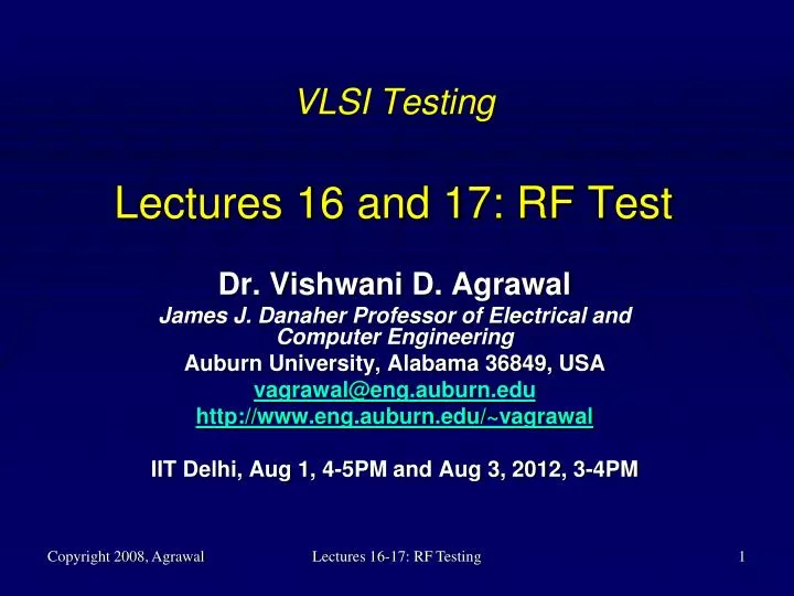
VLSI Testing Lectures 16 and 17: RF Test. Dr. Vishwani D. Agrawal James J. Danaher Professor of Electrical and Computer Engineering Auburn University, Alabama 36849, USA vagrawal@eng.auburn.edu http://www.eng.auburn.edu/~vagrawal IIT Delhi, Aug 1, 4-5PM and Aug 3, 2012, 3 -4PM. References.

E N D
VLSI TestingLectures 16 and 17: RF Test Dr. Vishwani D. Agrawal James J. Danaher Professor of Electrical and Computer Engineering Auburn University, Alabama 36849, USA vagrawal@eng.auburn.edu http://www.eng.auburn.edu/~vagrawal IIT Delhi, Aug 1, 4-5PM and Aug 3, 2012, 3-4PM Lectures 16-17: RF Testing
References S. Bhattacharya and A. Chatterjee, "RF Testing," Chapter 16, pages 745-789, in System on Chip Test Architectures, edited by L.-T. Wang, C. E. Stroud and N. A. Touba, Amsterdam: Morgan-Kaufman, 2008. M. L. Bushnell and V. D. Agrawal, Essentials of Electronic Testing for Digital, Memory & Mixed-Signal VLSI Circuits, Boston: Springer, 2000. J. Kelly and M. Engelhardt, Advanced Production Testing of RF, SoC, and SiP Devices, Boston: Artech House, 2007. B. Razavi, RF Microelectronics, Upper Saddle River, New Jersey: Prentice Hall PTR, 1998. J. Rogers, C. Plett and F. Dai, Integrated Circuit Design for High-Speed Frequency Synthesis, Boston: Artech House, 2006. K. B. Schaub and J. Kelly, Production Testing of RF and System-on-a-chip Devices for Wireless Communications, Boston: Artech House, 2004. Lectures 16-17: RF Testing
An RF Communications System Superheterodyne Transceiver ADC 0° Phase Splitter VGA LNA 90° ADC LO LO LO Duplexer Digital Signal Processor (DSP) DAC 0° PA VGA Phase Splitter 90° DAC RF IF BASEBAND Lectures 16-17: RF Testing
An Alternative RF Communications System Zero-IF (ZIF) Transceiver ADC 0° Phase Splitter LNA 90° ADC LO LO Duplexer Digital Signal Processor (DSP) DAC 0° Phase Splitter PA 90° DAC RF BASEBAND Lectures 16-17: RF Testing
Components of an RF System • Radio frequency • Duplexer • LNA: Low noise amplifier • PA: Power amplifier • RF mixer • Local oscillator • Filter • Intermediate frequency • VGA: Variable gain amplifier • Modulator • Demodulator • Filter • Mixed-signal • ADC: Analog to digital converter • DAC: Digital to analog converter • Digital • Digital signal processor (DSP) Lectures 16-17: RF Testing
LNA: Low Noise Amplifier • Amplifies received RF signal • Typical characteristics: • Noise figure 2dB • IP3 – 10dBm • Gain 15dB • Input and output impedance 50Ω • Reverse isolation 20dB • Stability factor > 1 • Technologies: • Bipolar • CMOS • Reference: Razavi, Chapter 6. Lectures 16-17: RF Testing
PA: Power Amplifier • Feeds RF signal to antenna for transmission • Typical characteristics: • Output power +20 to +30 dBm • Efficiency 30% to 60% • IMD – 30dBc • Supply voltage 3.8 to 5.8 V • Gain 20 to 30 dB • Output harmonics – 50 to – 70 dBc • Power control On-off or 1-dB steps • Stability factor > 1 • Technologies: • GaAs • SiGe • Reference: Razavi, Chapter 9. Lectures 16-17: RF Testing
Mixer or Frequency (Up/Down) Converter • Translates frequency by adding or subtracting local oscillator (LO) frequency • Typical characteristics: • Noise figure 12dB • IP3 +5dBm • Gain 10dB • Input impedance 50Ω • Port to port isolation 10-20dB • Tecnologies: • Bipolar • MOS • Reference: Razavi, Chapter 6. Lectures 16-17: RF Testing
LO: Local Oscillator • Provides signal to mixer for down conversion or upconversion. • Implementations: • Tuned feedback amplifier • Ring oscillator • Phase-locked loop (PLL) • Direct digital synthesizer (DDS) Lectures 16-17: RF Testing
SOC: System-on-a-Chip • All components of a system are implemented on the same VLSI chip. • Requires same technology (usually CMOS) used for all components. • Components not implemented on present-day SOC: • Antenna • Power amplifier (PA) Lectures 16-17: RF Testing
RF Tests • Basic tests • Scattering parameters (S-parameters) • Frequency and gain measurements • Power measurements • Power efficiency measurements • Distortion measurements • Noise measurements Lectures 16-17: RF Testing
Scattering Parameters (S-Parameters) • An RF function is a two-port device with • Characteristic impedance (Z0): • Z0 = 50Ω for wireless communications devices • Z0 = 75Ω for cable TV devices • Gain and frequency characteristics • S-Parameters of an RF device • S11 : input return loss or input reflection coefficient • S22 : output return loss or output reflection coefficient • S21 : gain or forward transmission coefficient • S12 : isolation or reverse transmission coefficient • S-Parameters are complex numbers and can be expressed in decibels as 20 × log | Sij | Lectures 16-17: RF Testing
Active or Passive RF Device a1 a2 Port 1 (input) RF Device Port 2 (output) b1 b2 Input return loss S11 = b1/a1 Output return loss S22 = b2/a2 Gain S21 = b2/a1 Isolation S12 = b1/a2 Lectures 16-17: RF Testing
S-Parameter Measurement by Network Analyzer Directional couplers DUT a1 Digitizer b1 Directional couplers a2 Digitizer b2 Lectures 16-17: RF Testing
Application of S-Parameter: Input Match • Example: In an S-parameter measurement setup, rms value of input voltage is 0.1V and the rms value of the reflected voltage wave is 0.02V. Assume that the output of DUT is perfectly matched. Then S11 determines the input match: • S11 = 0.02/0.1 = 0.2, or 20 × log (0.2) = –14 dB. • Suppose the required input match is –10 dB; this device passes the test. • Similarly, S22 determines the output match. Lectures 16-17: RF Testing
Gain (S21) and Gain Flatness • An amplifier of a Bluetooth transmitter operates over a frequency band 2.4 – 2.5GHz. It is required to have a gain of 20dB and a gain flatness of 1dB. • Test: Under properly matched conditions, S21 is measured at several frequencies in the range of operation: • S21 = 15.31 at 2.400GHz • S21 = 14.57 at 2.499GHz • From the measurements: • At 2.400GHz, Gain = 20×log 15.31 = 23.70 dB • At 2.499GHz, Gain = 20×log 14.57 = 23.27 dB • Result: Gain and gain flatness meet specification. Measurements at more frequencies in the range may be useful. Lectures 16-17: RF Testing
Power Measurements • Receiver • Minimum detectable RF power • Maximum allowed input power • Power levels of interfering tones • Transmitter • Maximum RF power output • Changes in RF power when automatic gain control is used • RF power distribution over a frequency band • Power-added efficiency (PAE) • Power unit: dBm, relative to 1mW • Power in dBm = 10 × log (power in watts/0.001 watts) • Example: 1 W is 10×log 1000 = 30 dBm • What is 2 W in dBm? Lectures 16-17: RF Testing
Harmonic Measurements Multiples of the carrier frequency are called harmonics. Harmonics are generated due to nonlinearity in semiconductor devices and clipping (saturation) in amplifiers. Harmonics may interfere with other signals and must be measured to verify that a manufactured device meets the specification. Lectures 16-17: RF Testing
Power-Added Efficiency (PAE) • Definition: Power-added efficiency of an RF amplifier is the ratio of RF power generated by the amplifier to the DC power supplied: • PAE = ΔPRF / PDC where • ΔPRF = PRF(output) – PRF(input) • Pdc = Vsupply× Isupply • Important for power amplifier (PA). • 1 – PAE is a measure of heat generated in the amplifier, i.e., the battery power that is wasted. • In mobile phones PA consumes most of the power. A low PAE reduces the usable time before battery recharge. Lectures 16-17: RF Testing
PAE Example • Following measurements are obtained for an RF power amplifier: • RF Input power = +2dBm • RF output power = +34dBm • DC supply voltage = 3V • DUT current = 2.25A • PAE is calculated as follows: • PRF(input) = 0.001 × 10²/10 = 0.0015W • PRF(output) = 0.001 × 1034/10 = 2.5118W • Pdc = 3× 2.25 = 6.75W • PAE = (2.5118 – 0.00158)/6.75 = 0.373 or 37.2% Lectures 16-17: RF Testing
Distortion and Linearity • An unwanted change in the signal behavior is usually referred to as distortion. • The cause of distortion is nonlinearity of semiconductor devices constructed with diodes and transistors. • Linearity: • Function f(x) = ax + b, although a straight-line is not referred to as a linear function. • Definition: A linear function must satisfy: • f(x + y) = f(x) + f(y), and • f(ax) = a f(x), for all scalar constants a Lectures 16-17: RF Testing
Linear and Nonlinear Functions f(x) f(x) slope = a b b x x f(x) = ax + b f(x) = ax2 + b f(x) slope = a x f(x) = ax Lectures 16-17: RF Testing
Generalized Transfer Function Electronic circuit vi vo • Transfer function of an electronic circuit is, in general, a nonlinear function. • Can be represented as a polynomial: • vo = a0 + a1 vi + a2 vi2 + a3 vi3 + · · · · • Constant term a0 is the dc component that in RF circuits is usually removed by a capacitor or high-pass filter. • For a linear circuit, a2 = a3 = · · · · = 0. Lectures 16-17: RF Testing
Effect of Nonlinearity on Frequency • Consider a transfer function, vo = a0 + a1 vi + a2 vi2 + a3 vi3 • Let vi = A cosωt • Using the identities (ω = 2πf): • cos2ωt = (1 + cos 2ωt)/2 • cos3ωt = (3 cosωt + cos 3ωt)/4 • We get, • vo = a0 + a2A2/2 + (a1A + 3a3A3/4) cosωt + (a2A2/2) cos 2ωt + (a3A3/4) cos 3ωt Lectures 16-17: RF Testing
Problem for Solution I V 0 – Is A diode characteristic is, I = Is ( eαV – 1) Where, V = V0 + vin, V0 is dc voltage and vin is small signal ac voltage. Isis saturation current and α is a constant that depends on temperature and design parameters of diode. Using the Taylor series expansion, express the diode current I as a polynomial in vin. Lectures 16-17: RF Testing
Linear and Nonlinear Circuits and Systems • Linear devices: • All frequencies in the output of a device are related to input by a proportionality, or weighting factor, independent of power level. • No frequency will appear in the output, that was not present in the input. • Nonlinear devices: • A true linear device is an idealization. Most electronic devices are nonlinear. • Nonlinearity in amplifier is undesirable and causes distortion of signal. • Nonlinearity in mixer or frequency converter is essential. Lectures 16-17: RF Testing
Types of Distortion and Their Tests • Types of distortion: • Harmonic distortion: single-tone test • Gain compression: single-tone test • Intermodulation distortion: two-tone or multitone test • Testing procedure: Output spectrum measurement Lectures 16-17: RF Testing
Harmonic Distortion • Harmonic distortion is the presence of multiples of a fundamental frequency of interest. N times the fundamental frequency is called Nth harmonic. • Disadvantages: • Waste of power in harmonics. • Interference from harmonics. • Measurement: • Single-frequency input signal applied. • Amplitudes of the fundamental and harmonic frequencies are analyzed to quantify distortion as: • Total harmonic distortion (THD) • Signal, noise and distortion (SINAD) Lectures 16-17: RF Testing
Problem for Solution Show that for a nonlinear device with a single frequency input of amplitude A, the nth harmonic component in the output always contains a term proportional to An. Lectures 16-17: RF Testing
Total Harmonic Distortion (THD) • THD is the total power contained in all harmonics of a signal expressed as percentage (or ratio) of the fundamental signal power. • THD(%) = [(P2 + P3 + · · · ) / Pfundamental ] × 100% • Or THD(%) = [(V22 + V32 + · · · ) / V2fundamental ] × 100% • Where P2, P3, . . . , are the power in watts of second, third, . . . , harmonics, respectively, and Pfundamental is the fundamental signal power, • And V2, V3, . . . , are voltage amplitudes of second, third, . . . , harmonics, respectively, and Vfundamental is the fundamental signal amplitude. • Also, THD(dB) = 10 log THD(%) • For an ideal distortionless signal, THD = 0% or – ∞ dB Lectures 16-17: RF Testing
THD Measurement • THD is specified typically for devices with RF output. • Separate power measurements are made for the fundamental and each harmonic. • THD is tested at specified power level because • THD may be small at low power levels. • Harmonics appear when the output power of an RF device is raised. Lectures 16-17: RF Testing
Gain Compression • The harmonics produced due to nonlinearity in an amplifier reduce the fundamental frequency power output (and gain). This is known as gain compression. • As input power increases, so does nonlinearity causing greater gain compression. • A standard measure of Gain compression is “1-dB compression point” power level P1dB, which can be • Input referred for receiver, or • Output referred for transmitter Lectures 16-17: RF Testing
Linear Operation: No Gain Compression Amplitude Amplitude time time LNA or PA Power (dBm) Power (dBm) frequency frequency f1 f1 Lectures 16-17: RF Testing
Cause of Gain Compression: Clipping Amplitude Amplitude time time LNA or PA Power (dBm) Power (dBm) frequency frequency f1 f1 f2 f3 Lectures 16-17: RF Testing
Effect of Nonlinearity • Assume a transfer function, vo = a0 + a1 vi + a2 vi2 + a3 vi3 • Let vi = A cosωt • Using the identities (ω = 2πf): • cos2ωt = (1 + cos 2ωt)/2 • cos3ωt = (3 cosωt + cos 3ωt)/4 • We get, • vo = a0 + a2A2/2 + (a1A + 3a3A3/4) cosωt + (a2A2/2) cos 2ωt + (a3A3/4) cos 3ωt Lectures 16-17: RF Testing
Gain Compression Analysis • DC term is filtered out. • For small-signal input, A is small • A2 and A3 terms are neglected • vo = a1A cos ωt, small-signal gain, G0 = a1 • Gain at 1-dB compression point, G1dB = G0 – 1 • Input referred and output referred 1-dB power: P1dB(output) – P1dB(input) = G1dB = G0 – 1 Lectures 16-17: RF Testing
1-dB Compression Point 1 dB Output power (dBm) 1 dB Compression point P1dB(output) Slope = gain Linear region (small-signal) Compression region P1dB(input) Input power (dBm) Lectures 16-17: RF Testing
Testing for Gain Compression • Apply a single-tone input signal: • Measure the gain at a power level where DUT is linear. • Extrapolate the linear behavior to higher power levels. • Increase input power in steps, measure the gain and compare to extrapolated values. • Test is complete when the gain difference between steps 2 and 3 is 1dB. • Alternative test: After step 2, conduct a binary search for 1-dB compression point. Lectures 16-17: RF Testing
Example: Gain Compression Test • Small-signal gain, G0 = 28dB • Input-referred 1-dB compression point power level, P1dB(input) = – 19 dBm • We compute: • 1-dB compression point Gain, G1dB = 28 – 1 = 27 dB • Output-referred 1-dB compression point power level, P1dB(output) = P1dB(input) + G1dB = – 19 + 27 = 8 dBm Lectures 16-17: RF Testing
Intermodulation Distortion Intermodulation distortion is relevant to devices that handle multiple frequencies. Consider an input signal with two frequencies ω1 and ω2: vi = A cosω1t + B cosω2t Nonlinearity in the device function is represented by vo = a0 + a1 vi + a2 vi2 + a3 vi3, neglecting higher order terms Therefore, device output is vo = a0 + a1 (A cosω1t + B cosω2t) DC and fundamental + a2 (A cosω1t + B cosω2t)2 2nd order terms + a3 (A cosω1t + B cosω2t)33rd order terms Lectures 16-17: RF Testing
Problems to Solve • Derive the following: vo = a0 + a1 (A cosω1t + B cosω2t) + a2 [ A2 (1+cos 2ω1t)/2 + AB cos (ω1+ω2)t + AB cos (ω1 – ω2)t + B2 (1+cos 2ω2t)/2 ] + a3 (A cosω1t + B cosω2t)3 • Hint: Use the identity: • cosαcosβ = [cos(α + β) + cos(α – β)] / 2 • Simplify a3 (A cosω1t + B cosω2t)3 Lectures 16-17: RF Testing
Two-Tone Distortion Products Order for distortion product mf1 ± nf2 is |m| + |n| Lectures 16-17: RF Testing
Problem to Solve Intermodulation products close to input tones are shown in bold. Lectures 16-17: RF Testing
Second-Order Intermodulation Distortion Amplitude Amplitude DUT f1 f2 f1 f2 2f1 2f2 f2 – f1 frequency frequency Lectures 16-17: RF Testing
Higher-Order Intermodulation Distortion Amplitude DUT Third-order intermodulation distortion products (IMD3) f1 f2 frequency 2f1 – f2 2f2 – f1 Amplitude f1 f2 2f1 2f2 3f1 3f2 frequency Lectures 16-17: RF Testing
Problem to Solve • For A = B, i.e., for two input tones of equal magnitudes, show that: • Output amplitude of each fundamental frequency, f1 or f2 , is 9 a1 A + — a3A3 ≈ a1 A 4 • Output amplitude of each third-order intermodulation frequency, 2f1 – f2 or 2f2 – f1 , is 3 — a3A3 4 Lectures 16-17: RF Testing
Third-Order Intercept Point (IP3) a1 A 3a3 A3 / 4 Output A IP3 • IP3 is the power level of the fundamental for which the output of each fundamental frequency equals the output of the closest third-order intermodulation frequency. • IP3 is a figure of merit that quantifies the third-order intermodulation distortion. • Assuming a1 >> 9a3 A2 /4, IP3 is given by a1 IP3 = 3a3 IP33 / 4 IP3 = [4a1 /(3a3 )]1/2 Lectures 16-17: RF Testing
Test for IP3 Select two test frequencies, f1 and f2, applied in equal magnitude to the input of DUT. Increase input power P0 (dBm) until the third-order products are well above the noise floor. Measure output power P1 in dBm at any fundamental frequency and P3 in dBm at a third-order intermodulationfrquency. Output-referenced IP3: OIP3 = P1 + (P1 – P3) / 2 Input-referenced IP3: IIP3 = P0 + (P1 – P3) / 2 = OIP3 – G Because, Gain for fundamental frequency, G = P1 – P0 Lectures 16-17: RF Testing
IP3 Graph OIP3 P1 f1 or f2 20 log a1 A slope = 1 2f1 – f2 or 2f2 – f1 20 log (3a3 A3 /4) slope = 3 Output power (dBm) P3 (P1 – P3)/2 P0 IIP3 Input power = 20 log A dBm Lectures 16-17: RF Testing
Example: IP3 of an RF LNA • Gain of LNA = 20 dB • RF signal frequencies: 2140.10MHz and 2140.30MHz • Second-order intermodulation distortion: 400MHz; outside operational band of LNA. • Third-order intermodulation distortion: 2140.50MHz; within the operational band of LNA. • Test: • Input power, P0 = – 30 dBm, for each fundamental frequency • Output power, P1 = – 30 + 20 = – 10 dBm • Measured third-order intermodulation distortion power, P3 = – 84 dBm • OIP3 = – 10 + [( – 10 – ( – 84))] / 2 = + 27 dBm • IIP3 = – 10 + [( – 10 – ( – 84))] / 2 – 20 = + 7 dBm Lectures 16-17: RF Testing