Image Pre-Processing

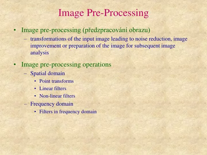
1. Image Pre-Processing • Image pre-processing (předzpracování obrazu) • transformations of the input image leading to noise reduction, image improvement or preparation of the image for subsequent image analysis • Image pre-processing operations • Spatial domain • Point transforms • Linear filters • Non-linear filters • Frequency domain • Filters in frequency domain

2. Point Transforms • Point transform (bodová transformace) • a pixel by pixel transformation of the image array in spatial domain • Position-dependent point transform g(x,y) = t ( f(x,y), x, y) t : < 0, NI >  < 0, Nx >  < 0, Ny >  < 0, NI > • Compensation for uneven illumination • Compensation for uneven dark charge of CCD pixels • Position-independent point transform g(x,y) = t ( f(x,y)) t : < 0, NI >  < 0, NI > • Change of image brightness: t (x) = x + k • Change of image contrast: t (x) = any function of x, for example: t (x) = k • x, t (x) = k • xn, t (x) = k • log(x), t (x) = k • exp(x)

3. Position-independent Point Transforms • Look-up table (LUT) • Usually t (x) is pre-computed, the table of its values is called look-up-table (LUT). The LUT is 1D array of values. The size of this array is determined by the bit depth of the image (256 values for 8-bit image, 4096 values for 12-bit image, etc.). • Intensity histogram • The best way to choose t (x) is to look at the intensity histogram of the given image. Intensity histogram is a 2D plot where x-axis represents intensity (e.g. 0-255 for 8-bit image) and y-axis represents the number of pixels in the image having the corresponding intensity.

4. Position-independent Point Transforms • Example of the influence of point transform (contrast change) on the intensity histogram for t (x) = 4 • x

5. Other Intensity Histogram Examples Under- and over-exposed image (pod- a pře-exponovaný obraz)

6. Filters • Filter (filtr) • a position-independent operator that transforms the image • Filter in spatial domain (filtr v prostorové doméně) • spatial operator that produces the output image array g(x,y)from the input image array f(x,y) • Filter in frequency domain (filtr ve frekvenční doméně) • frequency operator that produces the output image spectrum (x,y) from the input image spectrum F(x,y) • Low-pass filter (nízkofrekvenční filtr) • a filter that keeps low frequencies and suppresses the high ones • High-pass filter (vysokofrekvenční filtr) • a filter that keeps high frequencies and suppresses the low ones

7. Linear Filters • Linear filter (lineární filtr) • spatial linear operator that produces the output image array g(x,y) from the input image array f(x,y) in the following way: g(x0,y0) is obtained by a linear combination of pixels of the input image array f(x,y) within a neighbourhood of pixel (x0,y0). n=m=1: 3x3 neighbourhood n=m=2: 5x5 neighbourhood n=m=3: 7x7 neighbourhood

8. Linear Filters • Convolution kernel (konvoluční jádro) • The function h(a,b) is called convolution kernel. • The function h(a,b) is usually symmetric:h(a,b) = h(-a,b) = h(a,-b) = h(-a,-b). • The values of the function h(a,b) usually depend on radius: • The function h(a,b) is specified as a matrix H. • If n=m then the matrix H is square. g(x,y) = F(x,y) * H F(x,y) – matrix of neighbours of pixel (x,y) H – convolution kernel * – scalar matrix multiplication (defined in the same way as scalar vector multiplication)

9. Linear Filters Principle of linear filtering using a 3x3 convolution kernel • The intensity value at position (m,n) is replaced by the sum of nine numbers, where each number is obtained by multiplication of the number in matrix with the intensity value „behind“ this number. • This process (nine multiplications plus eight additions) must be performed for each position in the image, i.e. all values of m and n.

10. Linear Filters Problem with linear image filtering • Image convolution can be realised by scanning the convolution mask line by line over the image. At the shaded pixels the intensity value has already been replaced by the convolution sum. Thus the intensity values at the shaded pixels falling within the filter mask need to be stored in an extra buffer!

11. Smoothing Linear Filters • Smoothing (vyhlazování) • elimination of high frequencies • usually performed using averaging (either weighted or non-weighted) • Example: Smoothing using average 3x3 filters non-weighted weighted weighted

12. Smoothing Linear Filters • Gaussian filter (Gaussův filtr) • the best smoothing filter

13. Smoothing Linear Filters Example of Gaussian filtering with different values of s Original s = 1 s = 2 s = 4

14. Edge Detection Linear Filters • Edge detection (detekce hran) • usually performed using linear filters simulating 1st or 2nd derivative • can be used for edge enhancement or object boundaries reconstruction • Sobel filter • approximates the first derivative of the image • the basic kernels are (1,-1) or (1,0,-1) • mostly 3x3 kernel is used with the sum of coefficients equal to 0 • results for several 3x3 kernels can be averaged • there are 8 possibilities of the following type: • often used after Gaussian filter(so called derivative of Gaussian – DroG)

15. Edge Detection Linear Filters • Laplacian filter • approximates the second derivative of the image • the basic kernel is (1,-2,1) • mostly 3x3 kernel is used with the sum of coefficients equal to 0 • two basic types of 3x3 kernel are used, others are possible: • often used after Gaussian filter(so called Laplacian of Gaussian – LoG = Mexican hat filter)