Download
1 / 65
650 likes | 821 Views
STATE PLANE COORDINATE COMPUTATIONS Lectures 14 – 15 GISC-3325. Updates and details. Required reading assignments due 30 April 2008 Extra credit due 23 April 2008 Overdue lab assignments/homework will be given credit ONLY if received by 21 April 2008.

E N D
STATE PLANE COORDINATE COMPUTATIONS Lectures 14 – 15 GISC-3325
Updates and details • Required reading assignments due 30 April 2008 • Extra credit due 23 April 2008 • Overdue lab assignments/homework will be given credit ONLY if received by 21 April 2008. • Wednesday class: 16 April 2008 will be devoted to RTK. Mr. Toby Stock will demonstrate, make observations and show results. Meet him at Blucher during lecture and lab periods.
Datum: A set of constants specifying the coordinate system used to calculate coordinates of points on the Earth.
8 Constants • 3 to specify the origin. • 3 to specify the orientation. • 2 to specify the dimensions of the reference ellipsoid.
b a S a = Semi major axis b = Semi minor axis f = a-b = Flattening a N
BESSEL 1841 a = 6,377,397.155 m 1/f = 299.1528128 CLARKE 1866 a = 6,378,206.4 m 1/f = 294.97869821 GEODETIC REFERENCE SYSTEM 1980 - (GRS 80) a = 6,378,137 m 1/f = 298.257222101 WORLD GEODETIC SYSTEM 1984 - (WGS 84) a = 6,378,137 m 1/f = 298.257223563
Image on left from Geodesy for Geomatics and GIS Professionals by Elithorp and Findorff, OriginalWorks, 2004.
Map Projections From UNAVCO site hosting.soonet.ca/eliris/gpsgis/Lec2Geodesy.html
Conformal Mapping Projections • Mapping a curved Earth on a flat map must address possible distortions in angles, azimuths, distances or area. • Map projections where angles are preserved after projection are called “conformal”
http://www.cnr.colostate.edu/class_info/nr502/lg3/datums_coordinates/spcs.htmlhttp://www.cnr.colostate.edu/class_info/nr502/lg3/datums_coordinates/spcs.html
SPCS 27 designed in 1930s to facilitate the attachment of surveys to the national system. • Uses conformal mapping projections. • Restricts maximum scale distortion to less than 1 part in 10 000. • Uses as few zones as possible to cover a state. • Defines boundaries of zones on county-basis.
Source: http://www.cnr.colostate.edu/class_info/nr502/lg3/datums_coordinates/spcs.html
Secant cone intersects the surface of the ellipsoid NOT the earth’s surface.
d’ Ellipsoid c’ d c cd < c’d’ b b’ ab > a’b’ a a’ Grid Earth Center
Bs: Southern standard parallel (s) Bn: Northern standard parallel (n) Bb: Latitude of the grid origin (0) L0: Central meridian (0) Nb: “false northing” E0: “false easting” Constants were copied from NOAA Manual NOS NGS 5 (available on-line)
Zone constant computations Latitude of grid origin Mapping radius at equator. Equations from NGS manual, SPCS of 1983 NOS NGS 5
R0: Mapping radius at latitude of true projection origin. k0: Grid scale factor at CM. N0:Northing value at CM intersection with central parallel.
Convergence angle Grid scale factor at point. Conversion from geodetic coordinates to grid.
Distance = √(ΔE2+ΔN2) Azimuth =tan-1(ΔE / ΔN)
N.B. Convergence angle shown does NOT include the arc-to-chord correction.
STARTING COORDINATES • AZIMUTH • Convert Astronomic to Geodetic • Convert Geodetic to Grid (Convergence angle) • Apply Arc-to-Chord Correction (t-T) • DISTANCES • Reduction from Horizontal to Ellipsoidal • Elevation “Sea-Level” Reduction Factor • Grid Scale Factor
N = 3,078,495.629 E = 924,954.270 N = -25.13 k = 0.99994523 Convergence angle +01-12-19.0 LAPLACE Corr. -4.04 seconds
Laplace correction • Used to convert astronomic azimuths to geodetic azimuths. • A simple function of the geodetic latitude and the east-west deflection of the vertical at the ground surface. • Corrections to horizontal directions are a function of the Laplace correction and the zenith angle between stations, and can become significant in mountainous areas.
Astronomic to Geodetic Azimuth • = Φ – ξ • = Λ - (η / cos ) • α= A- η∙tan • (, ) are geodetic coordinates • (Φ, Λ) are astronomic coord. • (ξ, η) are the Xi and Eta corrections • (α, A) are geodetic and astronomic azimuths respectively)
Grid directions (t) are based on north being parallel to the Central Meridian. Remember: Geodetic and grid north ONLY coincide along CM.
Astronomic to Grid (via geodetic) ag = aA + Laplace Correction – g 253d 26m 14.9s - Observed Astro Azimuth + ( - 1.33s) - Laplace Correction 253d 26m 13.6s - Geodetic Azimuth + 1 12m 19.0s - Convergence Angle (g) 254d 38m 32.6s - Grid azimuth The convention of the sign of the convergence angle is always from Grid to Geodetic.
Arc-to-Chord correction δ (alias t – T) • Azimuth computed from two plane coordinate pairs is a grid azimuth (t). • Projected geodetic azimuth is (T). • Geodetic azimuth is (α ) • Convergence angle (γ) is the difference between geodetic and projected geodetic azimuths. • Difference between t and T = “δ”, the “arc-to-chord” correction, or “t-T” or “second-term” correction. • t = α-γ+ δ
Arc-to-Chord correction δ (alias t – T) Where t is grid azimuth.
When should it be applied? • Intended for during precise surveys. • Recommended for use on lines over 8 kilometers long. • It is always concave toward the Central Parallel of the projection. • Computed as: • δ = 0.5(sin 3-sin 0)(1- 2) • Where 3 = (21 + 2)/3
Compute magnitude of the second-term correction from preliminary coordinates. It is not significant for short sight distances (< 8km) but … The effect of this correction is cumulative!
Angle Reductions • Know the type of azimuth • Astronomic • Geodetic • Grid • Apply appropriate corrections • Angles (difference of two directions from a single station) do not need to consider convergence angle. • Apply arc-to-chord correction for long sight distances or long traverses (cumulative effect).
N1 = N + (Sg x cos ag) • E1 = E + (Sg x sin ag) • Where: • N = Starting Northing Coordinate • E = Starting Easting Coordinates • Sg = Grid Distance • ag = Grid Azimuth
Reduction of Distances • When working with geodetic coordinates use ellipsoidal distances. • When working with state plane coordinates reduce the observations to the grid (mapping surface).
Re is the radius of the Earth in the azimuth of the line. Lm is surface Le is ellipsoid
For most surveys the approximate radius used in NAD 27 (6,372,000 m or 20,906,000 ft) can be used for Re.