Download

1 / 29
300 likes | 564 Views
Intelligent Scissors for Image Composition. Anthony Dotterer 01/17/2006. Citation. Title Intelligent Scissors for Image Composition Author Eric N. Mortensen William A. Barrett Publication 1995. Intelligent Scissors Tool. Interactive image segmentation and composition tool Easy to use

E N D
Intelligent Scissors for Image Composition Anthony Dotterer 01/17/2006
Citation • Title • Intelligent Scissors for Image Composition • Author • Eric N. Mortensen • William A. Barrett • Publication • 1995
Intelligent Scissors Tool • Interactive image segmentation and composition tool • Easy to use • Quick • Quality output • Features • Best path along image edges • Cooling • On-the-fly training • Source to destination warping and composition • Destination matching
Intelligent Scissors • Need • Optimal path along edges starting at a ‘seed’ point • Optimal path creation must be quick • Solution • Use dynamic programming to create path reference • Local cost definition • Path reference creation
Local Cost Definition • Define l(p,q) as the cost for going from pixel p to pixel q • Incorporate the several edge functions into the cost • Laplacian Zero-Crossing, fZ(q) • Gradient Magnitude, fG(q) • Gradient Direction, fD (p,q) • Relate edge functions to the cost function • Use ωZ,ωD,ωGas constants to weight features l(p,q) = ωZ · fZ(q) + ωD · fD (p,q) + ωG · fG(q)
Laplacian Zero-Crossing • Properties • Approximate 2nd partial derivative of Image • Zero-crossings represent maxima and minima • Good image edges • Cost • Define IL(q) as Laplacian at pixel q • Get low cost by defining Laplacian as a binary fZ(q) = { 0; if IL(q) = 0, 1; if IL(q) ≠ 0
Laplacian Zero-Crossing (cont.) • Issue • Zeros rarely occur • Solution • Use pixel closest to zero • Examples • Image (top) • Laplacian (bottom)
Gradient Magnitude • Properties • Magnitude of 1st partial derivatives of an image • Direct correlation between edge strength and local cost • Cost • Define G as gradient magnitude G = √(Ix² + Iy²) • Get low cost by inverting and scaling fG = 1 – G / (max(G)) • Also factor in Euclidean distance • Scale adjacent pixels cost by 1 • Scale diagonal pixels cost by 1/√2
Gradient Magnitude (cont.) • Examples • Original (top left) • Gradient Magnitude (top right) • Inverted & Scaled Gradient Magnitude (bottom)
Gradient Direction • Properties • Vectors created by the 1st derivatives of an image • High cost for shape changes • Adds smoothing constraint • Cost • Give low costs to gradients in the same direction • Define D(p) as the unit vector perpendicular to the gradient vector at point p D(p) = norm(Iy(p), -Ix(p))
Gradient Direction (cont.) • Cost • Define L(p, q) to be the link between point q and p, such that L(p, q) = { q – p; if D(p) · (q – p) ≥ 0, p – q; if D(p) · (q – p) < 0 • Let dp(p, q) and dq(p, q) as follows dp(p, q) = D(p) · L(p, q) dq(p, q) = L(p, q) · D(q) • Finally, the cost function fD(p, q) = 1/π ( cos-1(dp(p, q)) + cos-1(dq(p, q)) )
Let p = (3, 3) q = (3, 4) D(p) = (0, 1) D(q) = (0, 1) Calculate L(p, q) L(p, q) = ((3, 4) – (3, 3)) = (0, 1) Determine d(p, q) dp(p, q) = (0, 1) · (0, 1) = 1 dq(p, q) = (0, 1) · (0, 1) = 1 Finally fD(p, q) fD(p, q) = 1/π ( 0 + 0 ) = 0 Low Cost! Let p = (3, 3) q = (4, 3) D(p) = (0, 1) D(q) = (0, 1) Calculate L(p, q) L(p, q) = ((4, 3) – (3, 3)) = (1, 0) Determine d(p, q) dp(p, q) = (0, 1) · (1, 0) = 0 dq(p, q) = (1, 0) · (0, 1) = 0 Finally fD(p, q) fD(p, q) = 1/π ( π/2 + π/2 ) = 1 High Cost! Gradient Direction (cont.)
Path Reference Creation • Differs from method studied in class • No stages • Link cost between nodes changes • No destination • Inputs • Seed point, s • Local cost function, l(q, r)
Path Reference Creation (cont.) • Data structures • Sorted list of active pixels, L • Neighborhood of pixel q, N(q) • Flag map of expanded pixels, e(q) • Cumulative cost from seed point, g(q) • Output • Path reference map, p
Path Reference Creation (cont.) • Start at seed point • Cost is adjusted for Euclidean distance • Put all neighbor pixels into the active list • No other pixel has yet to be expanded • Set pointers for all neighbors to the seed point 1 2 3 4 5 6 7 8 9 10 11 1 2 3 4 5 6 7 8 9 7 2 11 4 1 13 7 7 L = (4,8), (3,7), …
Path Reference Creation (cont.) • Expand to least cost node • Remove that node from active list • Calculate cumulative cost of all neighbor pixels • Excludes seed point • Change pointers of neighbor pixels • Only if new cost is smaller and pixel is not expanded • Add or replace neighbor pixels into active list • Do nothing if pointer was not updated 1 2 3 4 5 6 7 8 9 10 11 1 2 3 4 5 6 7 8 9 7 2 9 5 4 1 6 13 7 6 14 L = (3,7), (2,8), (5,7) …
Path Reference Creation (cont.) • Expand to least cost node • Remove that node from active list • Calculate cumulative cost of all neighbor pixels • Excludes expanded pixels • Change pointers of neighbor pixels • Only if new cost is smaller and pixel is not expanded • Add or replace neighbor pixels into active list • Do nothing if pointer was not updated 1 2 3 4 5 6 7 8 9 10 11 1 2 3 4 5 6 7 8 9 6 6 12 14 23 7 2 9 5 9 20 16 4 1 6 13 18 13 7 6 14 L = (2,6), (3,6), (4,9), …
Path Reference Creation (cont.) • Finished • No more pixels to expand • No more pixels on active list
‘Live-Wire’ Action • Mouse will constantly redraw optimal path • A wire will ‘snap’ to objects with an image • New seed points • New seed points must be defined to surround an object • Points will ‘snap’ to nearest edge
Cooling • Problem • All seeds must be manually selected • Complex objects may require many seed points • Solution • Apply automatic seed point • As the user wraps the object, a common path is formed • Make common path ‘cool’ into a new seed point
Cooling (cont.) • Examples • Manual seed points (bottom left) • Auto seed points via cooling (bottom right)
Interactive Dynamic Training • Problem • Some objects have stronger edges then others • If the desired edge is weaker than a nearby edge, then the path ‘jumps’ over to the stronger edge • Solution • Train the gradient magnitude to desire the weaker edge • Use a sample of good path to train gradient magnitude • Update sample as path moves along the desired edge • Allow user to enable and disable training as needed
Interactive Dynamic Training • Examples • Path segment jumps without training (top) • Path segment follows trained edge (middle) • Cost fG • Normal response without training (lower left) • Trained response from edge sample (lower right)
Image Composition • Need • Source objects need blend in with a new background • Background may need to be in front of objects • Solution • Allow for 2-D transformations to occur on source objects • Use low pass filters to blend the object into the destination’s scene • Mask background objects to appear in front of source object
Critique • Paper • Describes a tool • Selects image objects quickly and easily • Provides the means manipulate and paste them into different images • Abstract • Brief mention of need • List of abilities for a tool called ‘Intelligent Scissors’ • Introduction • Defines need • Claims current methods are not enough • Claims this tool will help the problem • Gives a small background on similar segmentation tools and their flaws
Critique (cont.) • Algorithms • The paper does a good job on explaining how dynamic programming is used • ‘Cooling’ was explained well, but no suggested times were given • The section on ‘Dynamic Training’ could be explained more to better understand it • Spatial Frequency and Contrast Matching needs more explanation
Critique (cont.) • Dynamic Programming • Used as the main driving force of this tool • The authors spend a lot of time on the dynamic programming section but not gratuitously • Cost must be correctly attributed to the different edge features to take advantage of dynamic programming • Optimal path is ‘Optimal’, not just a local answer