Download
1 / 18
270 likes | 427 Views
LIMITS An Introduction to Calculus. This presentation. LIMITS. What is Calculus? What are Limits? Evaluating Limits Graphically Numerically Analytically What is Continuity? Infinite Limits. Bring your graphing calculator to class!. Calculus. Precalculus Mathematics. Limit

E N D
This presentation LIMITS • What is Calculus? • What are Limits? • Evaluating Limits • Graphically • Numerically • Analytically • What is Continuity? • Infinite Limits Bring your graphing calculator to class!
Calculus Precalculus Mathematics Limit Process WHAT IS CALCULUS? • Calculus is • the mathematics of change • dynamic, whereas earlier mathematics is static • a limit machine As an example, an object traveling at a constant velocity can be modeled with precalculus mathematics. To model the velocity of an accelerating object, you need calculus.
TWO CLASSIC CALCULUS PROBLEMSthat illustrate how limits are used in calculus • The Tangent Line Problem Finding the slope of a straight line is a precalculus problem. . Finding the slope of a curve at a point, P, is a calculus problem. Q The limit process: Compute the slope of a line through P and another point, Q, on the curve. As the distance between the two points decreases, the slope gets more accurate. • The Area Problem Finding the area of a rectangle is a precalculus problem. Finding the area under a curve is a calculus problem. The limit process: Sum up the areas of multiple rectan-gular regions. As the number of rectangles increases (and their width decreases) the approximation improves. See other examples on pages 42-43 of your textbook.
The limit itself is a value of the function, i.e., its y value. In this case, the limit is L. Limits: An Informal Definition The limit is taken as the input, x, approaches a specific value from either side. In this case, x is approaching c. SO… If f(x) becomes arbitrarily close to a single number, L, as x approaches c from either side, then the limit of f(x) as x approaches c is L.
4 4 The existence or nonexistence of f(x) at c has nobearing on the existence of . In fact, even if , the limit can still exist. -5 -5 5 5 The existence or non-existence of f(x) at c has no bearing on the existence of . In fact, even if becomes arbitrarily close to a single number, L, as x approaches c from either side, the limit of f(x) as x approaches c is L. f(c) is undefined -4 -4 even though even though f(1) is undefined Limits: An Informal Definition If f(x) becomes arbitrarily close to a single number, L, as x approaches c from either side, the limit of f(x) as x approaches c is L. IMPORTANT POINT: f(c) ≠ L
Limits: Formal Definition The ε-δ definition of a limit: ε (epsilon) and δ (delta) are small positive numbers. means that x lies in the interval (c – δ, c + δ)i.e., 0 < |x – c| < δ. ↑ means x ≠ c means that f(x) lies in the interval (L – ε, L + ε)i.e., |f(x) – L| < ε. If f(x) becomes arbitrarily close to a single number, L, as x approaches c from either side, then the limit of f(x) as x approaches c is L. This formal definition is not used to evaluate limits. Instead, it is used to prove other theorems. FORMAL DEFINITION:Let f be a function on an open interval containing c (except possibly at c) and let L be a real number. The statement means that for each ε > 0, there exists a δ > 0 such that if 0 < |x – c| < δ, then |f(x) – L| < ε.
We will evaluate limits • Graphically • Numerically • Analytically
2. Evaluating Limits Graphically 1. What is ? What is ? (2, 6) (2, 6) a parabola a parabola w/ a hole in it Once again, the existence of a limit at a given point is independent of whether the function is defined at that point.
4 3. (-1, 2) -5 5 Even though f(-1) is undefined, is still 2. -4 Evaluating Limits Graphically (cont) This rational function is undefined at x = -1, because when x is -1, the denominator goes to zero. However, x = -1 is not a vertical asymptote* If you factor the numerator, you get Canceling like factors, you get This is a straight line. f(x) is still undefined at x = -1, so there is a hole in the graph at the point (-1, 2). * Rational functions can have point discontinuities as well as vertical asymptotes. If the rational expression can be simplified, the function is still not defined at this value of x, but the discontinuity becomes a point rather than a vertical line.
Draw the graph of a function such that . 4 4 4 f(3) is undefined f(3) = -1 -5 -5 -5 5 5 5 (3, 3) (3, -1) -4 -4 -4 (3, -1) Graph a function with a given limit Sketch any function that approaches (3, -1) from both directions. Simplest example is a straight line, e.g. f(x) = -x + 4. Three cases:
Limits that do not exist • Limits do not exist when: • f(x) approaches a different number from the right side of c than it approaches from the left side. • f(x) increases or decreases w/o bound as x approaches c. • f(x) oscillates between two fixed values as x approaches c. We will consider these cases graphically.
2 5. When x > 0, . Approaching zero from the right, . -2.5 2.5 (0, 1) (0, -1) Approaching from the left, . When x < 0, . -2 Evaluating Limits Graphically Limits that do not exist f(x) approaches a different number from the right side of c than it approaches from the left side. This function is undefined at x = 0, because the denominator goes to zero. This is called the right-hand limit. This is called the left-hand limit. When the behavior differs from right and left, the limit does not exist.
6. Evaluating Limits Graphically Limits that do not exist f(x) increases or decreases without bound as x approaches c. This function is undefined at x = 3, because the denominator goes to zero. It can not be simplified, so there is a vertical asymptote at x = 3. Approaching 3 from the right, f(x) increases without bound. Approaching 3 from the left, f(x) decreases without bound. When the function increases or decreases without bound, the limit does not exist.
We will evaluate limits • Graphically • Numerically • Analytically
Set . Graph the function. What happens to f(x) as x approaches 1 from the left and from the right? Use the TBLSET function. Set TblStart = 0.8 and set Tbl = 0.01. Go to the table. What happens as you move down the table from x = 0.8 to x = 1? Evaluating Limits Numerically Ex 1: Find We will do this using the Ti89 and its table function. Now set TblStart = 1.2. What happens as you move up the table from x = 1.2? In both cases, the f(x) values are getting closer and closer to 2, therefore
does not exist Set . Graph the function. What happens to f(x) as x approaches 3 from the left and from the right? Use the TBLSET function. Set TblStart = 2.8 and set Tbl = .01. Go to the table. What happens as you move down the table from x = 2.8 to x = 3? Evaluating Limits Numerically Ex 2: Find Now set TblStart = 3.2. What happens as you move up the table from x = 3.2? In both cases, f(x) values are growing without bound as x approaches 3 from the left and from the right. Therefore we say
LIMITS • Limits are a fundamental part of Calculus • The limit of a function at a specific input value, c, is the value of the function as you get increasingly closer to c. • The function need not be defined at this input value, c. • If the function is defined at c, the limit value and function value need not be the same. • Limits can be evaluated • Graphically, • Numerically, and • Analytically • Limits do not exist if, • The function approaches different values from the right and left • The function increases or decreases without bound • The function oscillates between 2 fixed values • Today, we focused on evaluating limits by studying the graphs of functions and numerically approaching x from both directions. • Next we will be evaluating limits analytically.