Download
1 / 62
620 likes | 689 Views
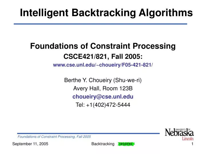
Intelligent Backtracking Algorithms. Foundations of Constraint Processing CSCE421/821, Fall 2005: www.cse.unl.edu/~choueiry/F05-421-821/ Berthe Y. Choueiry (Shu-we-ri) Avery Hall, Room 123B choueiry@cse.unl.edu Tel: +1(402)472-5444. Reading. Required reading

E N D
Intelligent Backtracking Algorithms Foundations of Constraint Processing CSCE421/821, Fall 2005: www.cse.unl.edu/~choueiry/F05-421-821/ Berthe Y. Choueiry (Shu-we-ri) Avery Hall, Room 123B choueiry@cse.unl.edu Tel: +1(402)472-5444 Backtracking
Reading • Required reading Hybrid Algorithms for the Constraint Satisfaction Problem [Prosser, CI 93] • Recommended reading • Chapters 5 and 6 of Dechter’s book • Tsang, Chapter 5 • Notes available upon demand • Notes of Fahiem Bacchus: Chapter 2, Section 2.4 • Handout 4 and 5 of Pandu Nayak (Stanford) Backtracking
Outline • Review of terminology of search • Hybrid backtracking algorithms • Looking ahead • Evaluation of (deterministic) BT search algorithms Backtracking
Backtrack search (BT) • Variable/value ordering • Variable instantiation • (Current) path • Current variable • Past variables • Future variables • Shallow/deep levels /nodes • Search space / search tree • Back-checking • Backtracking Backtracking
Outline • Review of terminology of search • Hybrid backtracking algorithms • Vanilla: BT • Improving back steps: {BJ, CBJ} • Improving forward step: {BM, FC} • Looking ahead • Evaluation of (deterministic) BT search algorithms Backtracking
Two main mechanisms in BT • Backtracking: • To recover from dead-ends • To go back • Consistency checking: • To expand consistent paths • To move forward Backtracking
Backtracking To recover from dead-ends • Chronological (BT) • Intelligent • Backjumping (BJ) • Conflict directed backjumping (CBJ) • With learning algorithms (Dechter Chapt 6.4) • Etc. Backtracking
Consistency checking To expand consistent paths • Back-checking: against past variables • Backmarking (BM) • Look-ahead: against future variables • Forward checking (FC) (partial look-ahead) • Directional Arc-Consistency (DAC) (partial look-ahead) • Maintaining Arc-Consistency (MAC) (full look-ahead) Backtracking
Hybrid algorithms Backtracking + checking = new hybrids • Evaluation: • Empirical: Prosser 93. 450 instances of Zebra • Theoretical: Kondrak & Van Beek 95 Backtracking
Notations (in Prosser’s paper) • Variables: Vi, i in [1, n] • Domain: Di = {vi1, vi2, …,viMi} • Constraint between Vi and Vj: Ci,j • Constraint graph: G • Arcs of G: Arc(G) • Instantiation order (static or dynamic) • Language primitives: list, push, pushnew, remove, set-difference, union, max-list Backtracking
Main data structures • v: a (1xn) array to store assignments • v[i] gives the value assigned to ith variable • v[0]: pseudo variable (root of tree), backtracking to v[0] indicates insolvability • domain[i]: a (1xn) array to store the original domains of variables • current-domain[i]: a (1xn) array to store the current domains of variables • Upon backtracking, current-domain[i] of future variables must be refreshed • check(i,j): a function that checks whether the values assigned to v[i] and v[j] are consistent Backtracking
Generic search: bcssp • Procedure bcssp (n, status) • Begin • consistent true • status unknown • i 1 • While status = unknown • Do Begin • If consistent • Then i label (i, consistent) • Else i unlabel (i, consistent) • If i > n • Then status “solution” • Else If i=0 then status “impossible” • End • End • Forward move: x-label • Backward move: x-unlabel • Parameters: current variable, Boolean • Return: new current variable Backtracking
Chronological backtracking (BT) • Uses bt-label and bt-unlabel • When v[i] is assigned a value from current-domain[i], we perform back-checking against past variables (check(i,k)) • If back-checking succeeds, bt-label returns i+1 • If back-checking fails, we remove the assigned value from current-domain[i], assign the next value in current-domain[i], etc. • If no other value exists, v[i-1] is un-instantiated and we seek a new value for it… (notation: in general v[h]) • For all future variables j: current-domain[j] = domain[j] • For all past variables g: current-domain[g] domain[g] Backtracking
BT-label • Function bt-label(i,consistent): INTEGER • BEGIN • consistent false • For v[i] each element of current-domain[i] while not consistent • Do Begin • consistent true • For h 1 to (i-1) While consistent • Do consistent check(i,h) • If not consistent • Then current-domain[i] remove(v[i], current-domain[i]) • End • If consistent then return(i+1) ELSE return(i) • END • Terminates: • consistent=true, return i+1 • consistent=false, current-domain[i]=nil, returns i Backtracking
BT-unlabel • FUNCTION bt-unlabel(i,consistent):INTEGER • BEGIN • h i -1 • current-domain[i] domain[i] • current-domain[h] remove(v[h],current-domain[h]) • consistent current-domain[h] nil • return(h) • END • Is called when consistent=false and current-domain[i]=nil • Selects vh to backtrack to • Uninstantiates all variables between vh and vi • Removes v[h] from current-domain [h] • Sets consistent to true if current-domain[h] 0 • Returns h Backtracking
Example: BT (the dumbest example ever) v[0] - {1,2,3,4,5} V1 v[1] 1 {1,2,3,4,5} v[2] V2 1 {1,2,3,4,5} V3 v[3] 1 CV3,V4={(V3=1,V4=3)} {1,2,3,4,5} etc… V4 v[4] 1 2 3 4 CV2,V5={(V2=5,V5=1),(V2=5,V5=4)} {1,2,3,4,5} V5 v[5] 1 2 3 4 5 Backtracking
Outline • Review of terminology of search • Hybrid backtracking algorithms • Vanilla: BT • Improving back steps: BJ, CBJ • Improving forward step: BM, FC • Looking ahead • Evaluation of (deterministic) BT search algorithms Backtracking
Danger of BT: thrashing • BT assumes that the instantiation of v[i] was prevented by a bad choice at (i-1). • It tries to change the assignment of v[i-1] • When this assumption is wrong, we suffer from thrashing (exploring ‘barren’ parts of solution space) • Backjumping (BT) tries to avoid that • Jumps to the reason of failure • Then proceeds as BT Backtracking
Backjumping (BJ) • Tries to reduce thrashing by saving some backtracking effort • When v[i] is instantiated, BJ remembers v[h], the deepest node of past variables that v[i] has checked against. • Uses: max-check[i], global, initialized to 0 • At level i, when check(i,h) succeeds max-check[i] max(max-check[i], h) • If current-domain[h] is getting empty, simple chronological backtracking is performed from h • BJ jumps then steps! 1 0 2 1 2 3 3 h-2 h-1 h h-1 h i 0 0 Past variable 0 Current variable Backtracking
1 0 2 1 2 3 3 h-2 h-1 h h-1 h i 0 0 0 BJ: label/unlabel • bj-label: same as bt-label, but updates max-check[i] • bj-unlabel, same as bt-unlabel but • Backtracks to h = max-check[i] • Resets max-check[j] 0 for j in [h+1,i] Important: max-check is the deepest level we checked against, could have been success or could have been failure Backtracking
{1,2,3,4,5} V1 {1,2,3,4,5} V2 CV2,V5={(V2=5,V5=1)} {1,2,3,4,5} V3 CV2,V4={(V2=1,V4=3)} {1,2,3,4,5} V4 CV1,V5={(V1=1,V5=2)} {1,2,3,4,5} V5 Example: BJ v[0] = 0 - v[1] Max-check[1] = 0 1 v[2] 1 2 Max-check[2] = 1 v[3] 1 V4=1, fails for V2, mc=2 V4=2, fails for V2, mc=2 V4=3, succeeds v[4] max-check[4] = 3 1 2 3 4 V5=1, fails for V1, mc=1 V5=2, fails for V2, mc=2 V5=3, fails for V1 v[5] V5=4, fails for V1 1 2 3 4 5 V5=5, fails for V1 max-check[5] = 2 Backtracking
Conflict-directed backjumping (CBJ) • Backjumping • jumps from v[i] to v[h], • but then, it steps back from v[h] to v[h-1] • CBJ improves on BJ • Jumps from v[i] to v[h] • And jumps back again, across conflicts involving both v[i] and v[h] • To maintain completeness, we jump back to the level of deepest conflict Backtracking
CBJ: data structure conf-set 0 • Maintains a conflict set: conf-set • conf-set[i] are first initialized to {0} • At any point, conf-set[i] is a subset of past variables that are in conflict with i 1 2 g conf-set[g] {0} h-1 {0} conf-set[h] h conf-set[i] {0} i {0} {0} {0} Backtracking
1 2 3 Past variables g {x, 3,1} {x} conf-set[g] h-1 {3} {3,1, g} conf-set[h] h Current variable i {1, g, h} conf-set[i] {0} {0} {0} CBJ: conflict-set • When a check(i,h) fails conf-set[i] conf-set[i] {h} • When current-domain[i] empty • Jumps to deepest past variable h in conf-set[i] • Updates conf-set[h] conf-set[h] (conf-set[i] \{h}) • Primitive form of learning (while searching) Backtracking
v[0] = 0 - V1 {1,2,3,4,5} v[1] conf-set[1] = {0} 1 V2 {1,2,3,4,5} conf-set[2] = {0} v[2] 1 {1,2,3,4,5} V3 v[3] conf-set[3] = {0} 1 {(V2=1,V4=3), (V2=4, V4=5)} v[4] 1 2 3 conf-set[4] = {1, 2} conf-set[4] = {2} {1,2,3,4,5} V4 {(V1=1,V5=3)} v[5] 1 2 3 conf-set[5] = {1} {1,2,3,4,5} v[6] 1 2 3 4 5 V5 conf-set[6] = {1} {(V4=5,V6=3)} conf-set[6] = {1} {1,2,3,4,5} conf-set[6] = {1,4} V6 {(V1=1,V6=3)} conf-set[6] = {1,4} conf-set[6] = {1,4} Example CBJ Backtracking
Backtracking: summary • Chronological backtracking • Steps back to previous level • No extra data structures required • Backjumping • Jumps to deepest checked-against variable, then steps back • Uses array of integers: max-check[i] • Conflict-directed backjumping • Jumps across deepest conflicting variables • Uses array of sets: conf-set[i] Backtracking
Outline • Review of terminology of search • Hybrid backtracking algorithms • Vanilla: BT • Improving back steps: BJ, CBJ • Improving forward step: BM, FC • Looking ahead • Evaluation of (deterministic) BT search algorithms Backtracking
k Backmarking: goal • Tries to reduce amount of consistency checking • Situation: • v[i] about to be re-assigned k • v[i] k was checked against v[h]g • v[h] has not been modified v[h] = g v[i] k Backtracking
v[h] = g v[h] = g k k v[i] k v[i] k BM: motivation • Two situations • Either (v[i]=k,v[h]=g) has failed it will fail again • Or, (v[i]=k,v[h]=g) was founded consistent it will remain consistent • In either case, back-checking effort against v[h] can be saved! Backtracking
max domain size m 0 0 0 0 0 0 0 0 0 Number of variables n 0 Number of variables n 0 0 0 Data structures for BM: 2 arrays • maximum checking level: mcl (n x m) • Minimum backup level: mbl (n x 1) Backtracking
max domain size m Number of variables n 0 0 0 0 0 0 0 0 0 0 0 0 0 Maximum checking level • mcl[i,k] stores the deepest variable that v[i]k checked against • mcl[i,k] is a finer version of max-check[i] Backtracking
Number of variables n Minimum backup level • mbl[i] gives the shallowest past variable whose value has changed since v[i] was the current variable • BM (and all its hybrid) do not allow dynamic variable ordering Backtracking
k When mcl[i,k]=mbl[i]=j BM is aware that • The deepest variable that (v[i] k) checked against is v[j] • Values of variables in the past of v[j] (h<j) have not changed So • We do need to check (v[i] k) against the values of the variables between v[j] and v[i] • We do not need to check (v[i] k) against the values of the variables in the past of v[j] v[j] v[i] k mbl[i] = j Backtracking
v[h] v[j] k v[i] k mcl[i,k] < mbl[i]=j mcl[i,k]=h Type a savings When mcl[i,k] < mbl[i], do not check v[i] k because it will fail Backtracking
k Type b savings When mcl[i,k] mbl[i], do not check (i,h<j) because they will succeed h v[j] v[g] v[i] k mcl[i,k]mbl[i] mcl[i,k]=g mbl[i] = j Backtracking
Hybrids of BM • mcl can be used to allow backjumping in BJ • Mixing BJ & BM yields BMJ • avoids redundant consistency checking (types a+b savings) and • reduces the number of nodes visited during search (by jumping) • Mixing BM & CBJ yields BM-CBJ Backtracking
v[m] v[g] v[g] v[h] v[h] v[h] v[i] v[i] Problem of BM and its hybrids: warning BMJ enjoys only some of the advantages of BM Assume: mbl[h] = m and max-check[i]=max(mcl[i,x])=g • Backjumping from v[i]: • v[i] backjumps up to v[g] • Backmarking of v[h]: • When reconsidering v[h], v[h] will be checked against all f in [m,g( • effort could be saved • Phenomenon will worsen with CBJ • Problem fixed by Kondrak & van Beek 95 v[m] v[m] v[f] v[g] v[h] v[i] Backtracking
Forward checking (FC) • Looking ahead: from current variable, consider all future variables and clear from their domains the values that are not consistent with current partial solution • FC makes more work at every instantiation, but will expand fewer nodes • When FC moves forward, the values in current-domain of future variables are all compatible with past assignment, thus saving backchecking • FC may “wipe out” the domain of a future variable (aka, domain annihilation) and thus discover conflicts early on. FC then backtracks chronologically • Goal of FC is to fail early (avoid expanding fruitless subtrees) Backtracking
v[i] v[k] v[m] v[j] v[l] v[n] FC: data structures • When v[i] is instantiated, current-domain[j] are filtered for all j connected to i and i<j<n • reduction[j] store sets of values remove from current-domain[j] by some variable before v[j] reductions[j] = {{a, b}, {c, d, e}, {f, g, h}} • future-fc[i]: subset of the future variables that v[i] checks against (redundant) future-fc[i] = {k, j, n} • past-fc[i]: past variables that checked against v[j] • All these sets are treated like stacks Backtracking
Forward Checking: functions • check-forward • undo-reductions • update-current-domain • fc-label • fc-unlabel Backtracking
FC: functions • check-forward(i,j) is called when instantiating v[i] • It performs REVISE(j,i) • Returns false if current-domain[j] is empty, true otherwise • Values removed from current-domain[j] are pushed, as a set, into reductions[j] • These values will be popped back if we have to backtrack over v[i] (undo-reductions) Backtracking
FC: functions • update-current-domain • current-domain[i] domain[i] \ reductions[i] • actually, we have to iterate over reductions=set of sets • fc-label • Attempts to instantiate current-variable • Then filters domains of all future variables (push into reductions) • Whenever current-domain of a future variable is wiped-out: • v[i] is un-instantiated and • domain filtering is undone (pop reductions) Backtracking
Hybrids of FC • FC suffers from thrashing: it is based on BT • FC-BJ: • max-check is integrated in fc-bj-label and fc-bj-unlabel • Enjoys advantages of FC and BJ… but suffers malady of BJ (jump the step) • FC-CBJ: • Best algorithm for far (assuming static variable ordering) • fc-cbj-label and fc-cbj-unlabel Backtracking
Consistency checking: summary • Chronological backtracking • Uses back-checking • No extra data structures • Backmarking • Uses mcl and mbl • Two types of consistency-checking savings • Forward-checking • Works more at every instantiation, but expands fewer subtrees • Uses: reductions[i], future-fc[i], past-fc[i] Backtracking
Experiments • Empirical evaluations on Zebra • Representative of design/scheduling problems • 25 variables, 122 binary constraints • Permutation of variable ordering yields new search spaces • Variable ordering: different bandwidth/induced width of graph • 450 problem instances were generated • Each algorithm was applied to each instance Experiments were carried out under static variable ordering Backtracking
Analysis of experiments Algorithms compared with respect to: • Number of consistency checks (average) FC-CBJ < FC-BJ < BM-CBJ < FC < CBJ < BMJ < BM < BJ < BT • Number of nodes visited (average) FC-CBJ < FC-BJ < FC < BM-CBJ < BMJ =BJ < BM = BT • CPU time (average) FC-CBJ < FC-BJ < FC < BM-CBJ < CBJ < BMJ < BJ < BT < BM FC-CBJ apparently the champion Backtracking
Additional developments • Other backtracking algorithms exist: • Graph-based backjumping (GBJ), etc. [Dechter] • Pseudo-trees [Freuder 85] • Other look-ahead techniques exist: • DAC, MAC, etc. • More empirical evaluations: • over randomly generated problems • Theoretical evaluations: • Based on approach of Kondrak & Van Beek IJCAI’95 Backtracking
Outline • Review of terminology of search • Hybrid backtracking algorithms • Looking ahead • Forward checking (FC) • Directional Arc Consistency (DAC) • Maintaining Arc Consistency (a.k.a. full arc-consistency) • Evaluation of (deterministic) BT search algorithms Backtracking
Looking ahead • Rationale: • As decisions are made (conditioning), • Revise the domain of future variables to propagate the effects of decisions • I.e., eliminate inconsistent choices in future sub-problem • Domain annihilation of a future variable avoids expansion of useless portions of the tree • Techniques • Partial: forward-checking (FC), directional arc-consistency (DAC) • Full: Maintaining arc-consistency (MAC) • Use: Revise(Vf, Vc), Vf future variable, Vc current variable Backtracking
Revising the domain of Vi • Revising the domain of Vi given a constraint C on Vi (i.e., ViScope(C)) • General notation: Revise(Vi,C) • In a binary CSP: Revise(Vi,C)= Revise(Vi,CVi,Vj)= Revise(Vi, Vj) Backtracking