Download
1 / 51
520 likes | 574 Views
Chapter 12: Indexing and Hashing. Basic Concepts Ordered Indices B+-Tree Index Files B-Tree Index Files Static Hashing Dynamic Hashing Comparison of Ordered Indexing and Hashing. Basic Concepts of Indexing. Speed up data access E.g., book indices

E N D
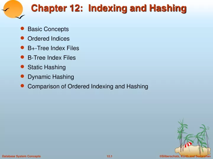
Chapter 12: Indexing and Hashing • Basic Concepts • Ordered Indices • B+-Tree Index Files • B-Tree Index Files • Static Hashing • Dynamic Hashing • Comparison of Ordered Indexing and Hashing
Basic Concepts of Indexing • Speed up data access • E.g., book indices • An index fileconsists of records (called index entries) of the form • Index files are typically much smaller than the original file • Two basic kinds of indices: • Ordered indices: search keys are stored in sorted order • Hash indices: search keys are distributed uniformly across “buckets” using a “hash function” pointer search-key
Index Evaluation Metrics • Access types supported efficiently. E.g., • records with a specified value in the attribute • records with an attribute value falling in a specified range of values. • Access time • Insertion time • Deletion time • Space overhead
Ordered Indices • Index entries are sorted by search key values • E.g., author catalog in library. • Primary index(clustering index) • the index whose search key specifies the sequential order of the file • Index-sequential files: files ordered on a primary index • The search key of a primary index is usually the primary key • Secondary index(non-clustering index) • An index whose search key specifies an order different from the sequential order of the file.
Dense Index Files • Dense index — Index record exists for every search-key value in the file.
Sparse Index Files • Sparse Index: contains index records for only some search-key values. • Applicable when records are sequentially ordered on search-key • To locate a record with search-key value K we: • Find index record with largest search-key value < K • Search file sequentially starting at the record to which the index record points • Less space and less maintenance overhead for insertions and deletions. • Slower than dense index for locating records. • Good tradeoff: sparse index with an index entry for every block in file, corresponding to least search-key value in the block.
Multilevel Index • If primary index does not fit in memory, access becomes expensive. • To reduce number of disk accesses to index records, treat primary index kept on disk as a sequential file and construct a sparse index on it. • outer index – a sparse index of primary index • inner index – the primary index file • If even outer index is too large to fit in main memory, yet another level of index can be created, and so on. • Indices at all levels must be updated on insertion or deletion from the file.
Index Update: Insertion/Deletion • Single-level index insertion: • Look up using the search-key value of the record to be inserted • Dense indices • If the search-key value does not appear in the index, insert it. • Sparse indices • If index stores an entry for each block of the file, no change needs to be made to the index unless a new block is created. • Single-level index deletion: • Dense indices • Sparse indices • Multilevel insertion (deletion) • Simple extensions of the single-level algorithms
Secondary Indices • To find all the records whose values in a certain field (which is not the search-key of the primary index) satisfy some condition • Example 1: In the account database stored sequentially by account number, we may want to find all accounts in a particular branch • Example 2: Find all accounts with a specified balance or range of balances • A secondary index with an index record for each search-key value • Index record points to a bucket that contains pointers to all the actual records with that particular search-key value
Primary and Secondary Indices • Secondary indices have to be dense. • Indices offer substantial benefits when searching for records • Compare to the sequential access without any index • When a file is modified, every index on the file must be updated - overhead • Sequential scan using primary index is efficient, but a sequential scan using a secondary index is expensive
B+-Tree Index Files • Disadvantage of indexed-sequential files • Performance degrades as file grows, since many overflow blocks get created. Periodic reorganization of the entire file is required. • B+-treeindex files: • Automatically reorganize with small, local changes during insertions and deletions. Reorganization of entire file is hardly required. • Disadvantage of B+-trees • Extra insertion and deletion overhead, space overhead. B+-tree indices are an alternative to indexed-sequential files.
B+-Tree Index Files (Cont.) • All paths from root to leaf are of the same length • Each node that is not a root or a leaf has between [n/2] and n children. • A leaf node has between [(n–1)/2] and n–1 values • Special cases: • If the root is not a leaf, it has at least 2 children. • If the root is a leaf (that is, there are no other nodes in the tree), it can have between 0 and (n–1) values. A B+-tree is a balanced tree satisfying the following properties:
B+-Tree Node Structure • Typical node • Ki are the search-key values • Pi are pointers to children (for non-leaf nodes) or pointers to records or buckets of records (for leaf nodes). • The search-keys in a node are ordered K1 < K2 < K3 < . . .< Kn–1
Leaf Nodes in B+-Trees Properties of a leaf node: • For i = 1, 2, . . ., n–1, pointer Pi either points to a file record with search key value Ki, or to a bucket of pointers to file records, each record having search-key value Ki. Only need bucket structure if search-key does not form a primary key. • If Li, Lj are leaf nodes and i < j, Li’s search-key values are less than Lj’s search-key values • Pn points to next leaf node in search-key order
Non-Leaf Nodes in B+-Trees • Non leaf nodes form a multi-level sparse index on the leaf nodes. For a non-leaf node with n pointers: • All the search-keys in the subtree to which P1 points are less than K1 • For 2 i n – 1, all the search-keys in the subtree to which Pi points have values greater than or equal to Ki–1 and less than Ki+1
Example of a B+-tree B+-tree for account file (n = 3)
Example of B+-tree • Leaf nodes must have between 2 and 4 values ((n–1)/2 and n –1, with n = 5). • Non-leaf nodes other than root must have between 3 and 5 children ((n/2 and n with n =5). • Root must have at least 2 children. B+-tree for account file (n - 5)
Observations about B+-trees • Since the inter-node connections are done by pointers, “logically” close blocks need not be “physically” close. • The non-leaf levels of the B+-tree form a hierarchy of sparse indices. • The B+-tree contains a relatively small number of levels (logarithmic in the size of the main file), thus searches can be conducted efficiently. • Why is this important? • Insertions and deletions to the main file can be handled efficiently, as the index can be restructured in logarithmic time (as we shall see).
Queries on B+-Trees • Find all records with a search key value of k. • Start with the root node • Examine the node for the smallest search key value > k. • If such a value Kj exists,follow Pi to the child node • Otherwise k Kn–1. Follow Pn to the child node. • If the node reached by following the pointer is not a leaf node, repeat the above procedure. • Eventually reach a leaf node. If for some i, key Ki = k follow pointer Pito the desired record or bucket. Else no record with search key value k exists.
Queries on B+-Trees (Cont.) • In processing a query, a path is traversed in the tree from the root to some leaf node. • If there are K search-key values in the file, the path is no longer than logn/2(K). • With 1 million search key values and n = 100, at most log50(1,000,000) = 4 nodes are accessed in a lookup. • A balanced binary tree with 1 million search key values — 20 nodes are accessed in a lookup • The difference is significant since every node access may need a disk I/O, costing around 20 milliseconds! • A node is generally the same size as a disk block, typically 4 kilobytes, and n is typically around 100 (40 bytes per index entry).
Updates on B+-Trees: Insertion • Find the leaf node to which the search key value should belong • If the search key value is already in the leaf node • Add the record to the file • Insert the pointer into the bucket • If the search key value is not there • Add the record to the file • If there is room in the leaf node, insert (key-value, pointer) pair in the leaf node • Otherwise, split the node
Updates on B+-Trees: Insertion (Cont.) • Splitting a node: • take the n(search-key value, pointer) pairs in sorted order. Place the first n/2 in the original node, and the rest in a new node. • let the new node be p, and let k be the least key value in p. Insert (k,p) in the parent of the node being split. If the parent is full, split it and propagate the split further up. • Splitting proceeds upwards till a node that is not full is found. In the worst case, split the root node, increasing the height of the tree by 1.
Updates on B+-Trees: Insertion (Cont.) B+-Tree before and after insertion of “Clearview”
Updates on B+-Trees: Deletion • Find the record to be deleted, and remove it from the file • Remove (search-key value, pointer) from the leaf node if there is no bucket or if the bucket has become empty • If the node has too few entries due to the removal, and the entries in the node and a sibling fit into a single node, then • Insert all the search-key values in the two nodes into a single node (the one on the left), and delete the other node. • Delete the pair (Ki–1, Pi), where Pi is the pointer to the deleted node, from its parent, recursively using the above procedure.
Updates on B+-Trees: Deletion • Otherwise, if the node has too few entries due to the removal, and the entries in the node and a sibling do NOT fit into a single node, then • Redistribute the pointers between the node and a sibling such that both have more than the minimum number of entries. • Update the corresponding search key value in the parent of the node. • The node deletions may cascade upwards till a node which has n/2 or more pointers is found. If the root node has only one pointer after deletion, it is deleted and the sole child becomes the root.
Examples of B+-Tree Deletion • The removal of the leaf node containing “Downtown” did not result in its parent having too little pointers. So the cascaded deletions stopped with the deleted leaf node’s parent. Before and after deleting “Downtown”
Examples of B+-Tree Deletion (Cont.) • Node with “Perryridge” becomes underfull (actually empty, in this special case) and merged with its sibling. • As a result “Perryridge” node’s parent became underfull, and was merged with its sibling (and an entry was deleted from their parent) • Root node then had only one child, and was deleted and its child became the new root node Deletion of “Perryridge” from result of previous example
Example of B+-tree Deletion (Cont.) Before and after deletion of “Perryridge” from earlier example
B+-Tree File Organization • Performance degradation problem of • index lookup: use B+-Tree indices • data file access: use B+-tree file organization • Let the leaf nodes in a B+-tree file organization store records (instead of pointers) • Insertion and deletion are handled in the same way as insertion and deletion of entries in a B+-tree index.
B+-Tree File Organization (Cont.) • Good space utilization is important • Records use more space than pointers. • To improve space utilization, involve more sibling nodes in redistribution during splits and merges • Involving 2 siblings in redistribution (to avoid split / merge where possible) results in each node having at least entries Example of B+-tree File Organization
B-Tree Index Files • B-tree allows search-key values to appear only once to eliminates redundant storage of search keys. • Advantages • May use less tree nodes than a corresponding B+-Tree. • Disadvantages: • Non-leaf nodes are larger, so fan-out is reduced. • B-Trees typically have greater depth • Insertion and deletion are more complicated. • Implementation is harder. • Typically, advantages of B-Trees do not out weigh disadvantages.
Static Hashing • A bucket is a unit of storage containing one or more records (a bucket is typically a disk block). • In a hash file organization we obtain the bucket of a record directly from its search-key value using a hashfunction. • Hash function h is a function from the set of all search-key values K to the set of all bucket addresses B. • Hash function is used to locate records for access, insertion as well as deletion. • Records with different search-key values may be mapped to the same bucket; thus entire bucket has to be searched sequentially to locate a record.
Example of Hash File Organization (Cont.) • There are 10 buckets, • The binary representation of the ith character is assumed to be the integer i. • The hash function returns the sum of the binary representations of the characters modulo 10 • E.g. h(Perryridge) = 5 h(Round Hill) = 3 h(Brighton) = 3 Hash file organization of account file, using branch-name as key (See figure in next slide.)
Example of Hash File Organization Hash file organization of account file, using branch-name as key (see previous slide for details).
Hash Functions • Ideal hash function • Uniform: each bucket is assigned the same number of search key values from the set of all possible values. • Random: each bucket will have the same number of records assigned to it irrespective of the actual distribution of search key values in the file. • Typical hash functions perform computation on the internal binary representation of the search-key • Add the binary representations of all the characters in the string • Return (sum % number of buckets)
Handling of Bucket Overflows • Bucket overflow can occur because of • Insufficient buckets • Skew in distribution of records. This can occur due to two reasons: • chosen hash function produces non-uniform distribution of key values • multiple records have same search key value • Although the probability of bucket overflow can be reduced, it cannot be eliminated; it is handled by using overflow buckets.
Handling of Bucket Overflows (Cont.) • Overflow chaining (closed hashing) • Overflow buckets of a given bucket are chained together in a linked list. • Linear probing
Deficiencies of Static Hashing • In static hashing, function h maps search-key values to a fixed set of B of bucket addresses. • Databases grow with time. If initial number of buckets is too small, performance will degrade due to too much overflows. • If file size at some point in the future is anticipated and number of buckets allocated accordingly, significant amount of space will be wasted initially. • If database shrinks, again space will be wasted. • One option is periodic re-organization of the file with a new hash function, but it is very expensive. • Allow the number of buckets to be modified dynamically.
Extendible Hashing • Situation: Bucket becomes full. Why not re-organize file by doubling # of buckets? • Reading and writing all pages is expensive! • Idea: Use directory of pointers to buckets, double # of buckets by doubling the directory, splitting just the bucket that overflowed! • Directory much smaller than file, so doubling it is much cheaper. Only one page of data entries is split. Nooverflowpage! • Trick lies in how hash function is adjusted!
Example LOCAL DEPTH 2 Bucket A 16* 4* 12* 32* GLOBAL DEPTH • Directory is array of size 4. • To find bucket for r, take last `global depth’ # bits of h(r); we denote r by h(r). • If h(r) = 5 = binary 101, it is in bucket pointed to by 01. 2 2 Bucket B 00 5* 1* 21* 13* 01 2 10 Bucket C 10* 11 2 DIRECTORY Bucket D 15* 7* 19* DATA PAGES • Insert: If bucket is full, splitit (allocate new page, re-distribute). • If necessary, double the directory. (As we will see, splitting a • bucket does not always require doubling; we can tell by • comparing global depth with local depthfor the split bucket.)
Insert h(r)=20 (Causes Doubling) 2 LOCAL DEPTH 3 LOCAL DEPTH Bucket A 16* 32* 32* 16* GLOBAL DEPTH Bucket A GLOBAL DEPTH 2 2 2 3 Bucket B 5* 21* 13* 1* 00 1* 5* 21* 13* 000 Bucket B 01 001 2 10 2 010 Bucket C 10* 11 10* Bucket C 011 100 2 2 DIRECTORY 101 Bucket D 15* 7* 19* 15* 7* 19* Bucket D 110 111 2 3 Bucket A2 4* 12* 20* DIRECTORY 12* 20* Bucket A2 4* (`split image' of Bucket A) (`split image' of Bucket A)
Points to Note • 20 = binary 10100. Last 2 bits (00) tell us r belongs in A or A2. Last 3 bits needed to tell which. • Global depth of directory:Max # of bits needed to tell which bucket an entry belongs to. • Local depth of a bucket:# of bits used to determine if an entry belongs to this bucket. • When does bucket split cause directory doubling? • Before insert, local depth of bucket = global depth. Insert causes local depth to become > global depth; directory is doubled by copying it overand `fixing’ pointer to split image page. (Use of least significant bits enables efficient doubling via copying of directory!)
Directory Doubling • Why use least significant bits in directory? • Allows doubling via copying! 6 = 110 6 = 110 3 3 000 000 001 100 2 2 010 010 00 00 1 1 011 110 6* 01 10 0 0 100 001 6* 6* 10 01 1 1 101 101 6* 11 11 6* 6* 110 011 111 111 vs. Least Significant Most Significant
Comments on Extendible Hashing • If directory fits in memory, equality search answered with one disk access; else two. • 100MB file, 100 bytes/rec & 4K pages, contains 1,000,000 records (as data entries) and 25,000 directory elements; chances are high that directory will fit in memory. • Directory grows in spurts, and, if the distribution of hash values is skewed, directory can grow large. • Multiple entries with same hash value cause problems! • Delete: If removal of data entry makes bucket empty, can be merged with `split image’. If each directory element points to same bucket as its split image, can halve directory.
Extendable Hashing vs. Other Schemes • Benefits of extendable hashing: • Hash performance does not degrade with growth of file • Minimal space overhead • Disadvantages of extendable hashing • Extra level of indirection to find desired record • Bucket address table may itself become very big (larger than memory) • Need a tree structure to locate desired record in the structure! • Changing size of bucket address table is an expensive operation • Linear hashing is an alternative mechanism which avoids these disadvantages at the possible cost of more bucket overflows
Comparison of Ordered Indexing and Hashing • Frequency of insertions and deletions • Cost of periodic re-organization • Is it desirable to optimize average access time at the expense of worst-case access time? • Expected type of queries: • Hashing is generally better at retrieving records having a specified value of the key. • If range queries are common, ordered indices are to be preferred