Download
1 / 31
320 likes | 569 Views
BREAKEVEN ANALYSIS. Introduction What is Break-even Analysis? Break-even in comparing alternative propositions Break-even in single project analysis Break-even in decision making Optimisation. INTRODUCTION. Break-even analysis – a powerful management tool A tool for cost comparison

E N D
BREAKEVEN ANALYSIS Introduction What is Break-even Analysis? Break-even in comparing alternative propositions Break-even in single project analysis Break-even in decision making Optimisation
INTRODUCTION • Break-even analysis – a powerful management tool • A tool for cost comparison • Example: How can we choose between two different options for a required piece of equipment? • A tool for single project analysis • Example: How many units are required to be sold before the project yields a positive profit? • A tool for decision making • Example: is an investment in a marketing initiative that is believed to have a certain benefit worth undertaking?
COMPARING ALTERNATIVES • In situations where the alternatives are affected in some way by a common variable • Total cost of Option 1 = TC1 • Total cost of Option 2 = TC2 • There exists a common, independent decision variable affecting both Options – ‘x’
EQUIPMENT SELECTION EXAMPLE • 2 pump options • Electric: Capital cost + Annual maintenance + Energy cost • Diesel: Capital cost + Hourly maintenance + Hourly operator cost + Energy cost • 4 year project life • 12% interest rate • Which is the lowest cost option?
PROBLEM SOLVING PROCESS • Identify the common, independent decision variable • Translate the cost information for each option into cost function form • Do the number crunching • Solve analytically or graph both cost functions • Locate the break-even value (the intersection of the two cost functions)
SOLUTION 1 • Common, independent decision variable • ‘h’, pump operational hours per year • Cost function for Pump 1 • Initial cost Annual Equivalent • Annual maintenance cost Annual amount • Energy cost Hourly rate • Cost function for Pump 2 • Initial cost Annual Equivalent • Maintenance cost Hourly rate • Energy cost Hourly rate • Operator cost Hourly rate
SOLUTION 2 • Common cost function: Total Annual Equivalent Cost = Annual Cost + Hourly Rate * h • Equation of a straight line y (TAEC) = m (Hourly rate). x (h) + c (Annual cost) • Result is two straight lines, one for each option
SOLUTION 3 – NUMBER CRUNCHING • Pump 1 Initial Capital cost = 1,800 m.u. Annual Equivalent = Initial Cost * A/P(12,4) = 1,800 * 0.3292 = 592.56 m.u. Annual maintenance cost = 360.00 m.u. Total Annual cost = 952.56 m.u. Hourly rate = 1.10 m.u. / hour Total Annual Equivalent cost = 952.56 + 1.10*h ………(1)
SOLUTION 4 – NUMBER CRUNCHING • Pump 2 Initial Capital cost = 550 m.u. Annual Equivalent = Initial Cost * A/P(12,4) = 550 * 0.3292 Total Annual cost = 181 m.u. Hourly rate = 0.60 + 1.40 + 0.35 m.u. / hour = 2.35 m.u. / hour Total Annual Equivalent cost = 181.00 + 2.35*h ………(2)
SOLUTION 5 – SOLVE • Analytical • Total Annual Equivalent cost = 952.56 + 1.10*h ………(1) • Total Annual Equivalent cost = 181.00 + 2.35*h ………(2) • Break-even is when these are equal, i.e. 952.56 + 1.10*h = 181.00 + 2.35*h 771.56 = 1.25*h h = 617.25
MULTIPLE – ALTERNATIVE PROBLEMS • The same solution approach applies • Reduce all problems to common cost function • Graphical solution is best way of visualising the solution V < 50 Blue 50 < V < 150 Green 150 < V Red
BREAK-EVEN IN A SINGLE PROJECT • Definition of Costs • Fixed: “A cost is said to be fixed if it does not change in response to changes in the level of activity” • Variable: “The cost that is directly associated with the production of one unit” Total Cost Total Cost (Ct) Cv Cf Volume (v)
COST – VOLUME – PROFIT EXAMPLE • Telephone: Annual line rental charge 25.00 m.u. Cost per call 0.10 m.u. • Cost for 100 calls Line rental + call cost 35.00 m.u. [0.35] • Cost for 500 calls Line rental + call cost 75.00 m.u. [0.25] Total Cost (Ct) Average Cost “Average cost is the total cost of providing a product or service, divided by the number that are provided.” 75 35 25 500 100 Volume (v)
LINEARITY OF VARIABLE COSTS • Variable costs = f (volume), but the relationship is not linear • Limitations on linearity • Bulk purchase price break point • Demand fluctuations • Economic climate • Production capability • Efficiency & Productivity changes • Technology changes
REALISTIC COST FUNCTIONS Fixed Cost Variable Cost + Volume Volume Total Cost = Relevant Range Volume
CVP ANALYSIS • Profit (P) = Sales Revenue (SR) – Total Costs (Ct) • SR = Selling Price (Sp) * Volume (V) • Ct = Fixed Costs (Cf) + Variable Costs (CV) • Marginal cost: “The cost of providing one additional unit/item • Cv = Marginal Cost (Cv) * Volume • Break-even when P=0
BREAK-EVEN ANALYSIS Profit Gradient = (Sp - Cv) At Breakeven P = 0 Cf Break-Even Volume Volume
SINGLE PRODUCT DECISIONS • You buy and sell a product which sells for 15.00 m.u. each. The cost for you to purchase the product is 3.00 m.u. In order for you to trade you require premises and equipment which, in total, represent a fixed cost to you of 25,000 m.u. Your total planned volume for the year of the product is 4,000 units. • How many units do you need to sell to break-even? • How many units do you need to sell to make 1,000 m.u. profit? • Would it be worth the introduction of advertising at a cost of 6,000 m.u. to increase sales to 4,450? • What impact would a 10% drop in selling price have on the break-even volume?
SOLUTION - 1 Problem 1) How many units to breakeven? P = (Sp - Cv) * V - Cf Definition of Break-Even : P = 0 Profit Break-Even Volume = 2084 £25k Break-Even Volume = 2083.3
SOLUTION - 2 Problem 2) How many units to make £1000 profit? P = (Sp - Cv) * V - Cf Volume for Profit = £1000 Profit Volume = 2167 £26k Volume = 2166.6
SOLUTION - 3 Problem 3) Would it be worth the introduction of advertising at a cost of £6,000 to increase sales to 4450? P = (Sp - Cv) * V - Cf Profit for V = 4000 is £23,000 Profit for V = 4450 is £28,400 Gain in Profit = £5,400 Cost to Achieve Gain = £6,000 Hence Not Worth Pursuing!
SOLUTION - 4 Problem 4) What impact would a 10% drop in selling price have on the break even volume. ? P = (Sp - Cv) * V - Cf Profit Increase = 298 units or 14.3% £25k Break-Even Volume = 2381
CONTRIBUTION Problem 3) Would it be worth the introduction of advertising at a cost of £6,000 to increase sales to 4450? P = (Sp - Cv) * V - Cf Profit for V = 4000 is £23,000 Profit for V = 4450 is £28,400 Gain in Profit = £5,400 Cost to Achieve Gain = £6,000 There is an alternative way of solving this.
CONTRIBUTION Problem 3) Would it be worth the introduction of advertising at a cost of £6,000 to increase sales to 4450? P = (Sp - Cv) * V - Cf Per unit Profit = (Sp - Cv) = £12 Increase in Volume with Advertising : 450 units Increase in Profit = £12 * 450 = £5,400 Cost to Achieve Gain = £6,000 “£12 is the contribution or profit margin per unit”
Revenue / Cost Sales Revenue Contribution Cf Variable Costs Volume CONTRIBUTION Marginal Contribution = Selling Price - Variable Cost Total Contribution = (Selling Price - Variable Cost) * Volume
OPTIMISATION ANALYSIS • Some cost components vary directly with a common decision variable while others vary inversely with the decision variable • In such cases an optimum (lowest cost) exists • The general form of such a cost function is: • Where: • x = common decision variable • TC = Total cost • A, B, C = constants
OPTIMISATION ANALYSIS • The general form can be solved analytically and/or graphically
ALTERNATIVE OPTIONS - 1 • Single cross-over • Lowest cost option changes once
ALTERNATIVE OPTIONS - 2 • Double cross-over • Lowest cost option changes twice
ALTERNATIVE OPTIONS - 3 • No cross-overs • Lowest cost option never changes
OPTIMISATION CASE STUDY Sometown Compressors