Download
1 / 30
300 likes | 425 Views
Scalable Low Overhead Delay Estimation. Yossi Cohen Advance IP seminar. Topics viewed. IP inefficiency with multiple receivers Multicast overview Multicast delay (RTT) estimation problems Proposed solution. “ TV ” on the web .

E N D
Scalable Low Overhead Delay Estimation Yossi Cohen Advance IP seminar
Topics viewed • IP inefficiency with multiple receivers • Multicast overview • Multicast delay (RTT) estimation problems • Proposed solution
“TV” on the web • What happens when there is a broadcast of the same data to many users (thousands)? • Example : “Madonna online” last month on msn.
The problem • Congestion
Result • Buffering…. • Site is overloaded try later…
Multicast Overview IGMP & SRM
IP Multicast-basic ideas • The last routers before a path split would duplicate the packets. • The packets travel once instead of thousands of times (flash). • Supported by most routers made in the last years (need SW upgrade).
IP Multicast – Advantages/ Disadvantages • Advantages • Less congestion. • Reduce unicast servers load. • Disadvantages • Not reliable (Like UDP) • Needs application that support it.
Why Multicast is not used? • Billing – How should ISPs bill a multicast session? • Application support. • Access rights/Security. • Since some routers don’t support it there (old routers or not enabled new routers) there would always be a need for hybrid unicast multicast (HMU). So why not use unicast only.
IGMP • Internet Group Management Protocol • The basic Multicast protocol. • Described in RFC2933. • IP Layer level protocol (with ICMP) • Carried in IP datagrams.
IGMP • IGMP defines the multicast group interfaces and the protocols for joining and leaving a multicast group. • Two types of messages: Host message and Router message. • Defines a special group address
Problems with IGMP • IP is a “Best effort” protocol which does not guarantee that the information sent was actually received by the client. • Therefore IGMP is unreliable.
Reliability in multicast • Several algorithms were proposed to solve this problems and create are more reliable Multicast. • SRM, MTCP (Multicast TCP) and RMTP (Reliable Multicast Transport protocol) are “TCP-like” protocol for multicast networks that tries to guarantee delivery.
Scalable low overhead network delay estimation Problem definition Network Model BW estimation
In multicast we trust? • In order to evaluate the network bandwidth TCP estimates the RTT. (used in “Window Size” coeff.) • SRM and other “Reliable Multicast” protocols also need accurate and low bandwidth delay estimation method in order to work properly.
Problem definition • “Reliable” multicast protocols needs an accurate low bandwidth delay estimation from each node to each node in a multicast network. • Current methods cost high BW according to the authors multicast network model (Would be calculated soon). • This article suggest a methods to get accurate results with lower bandwidth.
Network Model • This article assumes a FULL multicast network in which each node multicast to all the others. A clique model.
Model correctness • Most application that use multicast are working in a few->many (forest model) method for example video conferencing, company broadcast, Distance learning etc. • See examples at RealM. • this multicast model and the calculation derived from it are not correct.
(Remarks) • So what have we done? • Current multicast application and their delay estimation protocols are built for a tree/forest model. The article assumes a model that is not used in neither MIB application (VC, DL, broadcast), say there is a huge overhead and try to correct it. If it was truly such a huge overhead don’t you think it would be corrected by now ?! Anyway let’s continue…
BW estimation-Suggested protocol • Current protocol aim to lower the bandwidth needed to 10KB/S which could be acceptable.
Current method – How they work • SRM uses a protocol called session to estimate delay. • Each node periodically multicast last time-stamps received from other nodes. • So each node multicast O(n) timestamps totaling in O(n^2). (according to the network model)
What is suggested? n^2 n (only for delay estimation basic config. stays the same) R
(Remarks) • If we look at this model closely and redraw it it is easy to see that the “new” network configuration suggested was actually the tree model…..
Further explanation • One node would be used as a “Reference point”. • Each node send a message to the reference point o(n) and then it multicast all timestamps received to all the nodes o(n) again. So BW consumption is o(n). • This however is not enough to estimate delay between any node to any node.
The Delay estimation protocol Set-up Node-Node delay estimation
Set-up phase • In this phase each node Q determines the delay from the reference point S to itself, d(q,s). • In order to do that it send it’s current time to the reference point S. S sends the message back with it’s time stamp. • By using the time-stamp diff Q can compute d(Q,S) S R Q
Delay estimation phase • In this phas each node R determines the delay from each node Q to itself. • d(Q,R) = d(Q,S)+d(S,R) + dmM – (tM-tm) • Explanation:Node Q multicast a probe message containing d(Q,S) (determined in set-up phase) and the local time it send it m. • Tm is the time that node R receives the message. S R Q
Delay estimation phase-continues • Upon receiving m S multicast M containing tmM the time between receiving and sending m. • froom this we receive • d(Q,R) = d(Q,S)+d(S,R) + dmM – (tM-tm)
Time is relative - proof • Let t be the time(in R’s clock) that Q sent message m. • Since m was received in R at tm then t = tm – d(Q,R). • Also since M was received in tM then t = tM – d(S,R)-dmM-d(Q,S) • tm – d(Q,R) = tM – d(S,R)-dmM-d(Q,S) • d(Q,R) = d(Q,S)+d(S,R) + dmM – (tM-tm)
Summery • For each d(Q,R) we used two multicast messages (after the set-up phase). This reduce the BW used to estimate delay from o(n^2) to o(n).