Download
1 / 54
540 likes | 714 Views
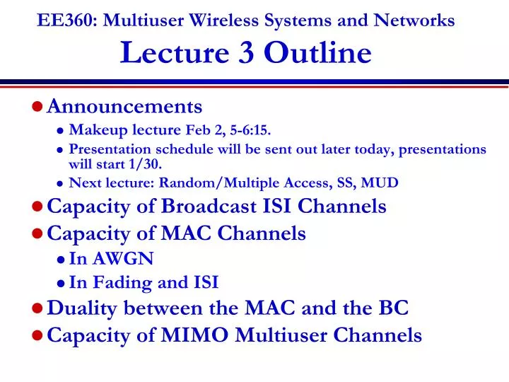
EE360: Multiuser Wireless Systems and Networks Lecture 3 Outline. Announcements Makeup lecture Feb 2, 5-6:15. Presentation schedule will be sent out later today, presentations will start 1/30. Next lecture: Random/Multiple Access, SS, MUD Capacity of Broadcast ISI Channels

E N D
EE360: Multiuser Wireless Systems and NetworksLecture 3 Outline • Announcements • Makeup lecture Feb 2, 5-6:15. • Presentation schedule will be sent out later today, presentations will start 1/30. • Next lecture: Random/Multiple Access, SS, MUD • Capacity of Broadcast ISI Channels • Capacity of MAC Channels • In AWGN • In Fading and ISI • Duality between the MAC and the BC • Capacity of MIMO Multiuser Channels
g1(t) g2(t) g3(t) x x x Review of Last Lecture Broadcast: One Transmitter to Many Receivers. R3 R2 R1 • Channel capacity region of broadcast channels • Capacity in AWGN • Use superposition coding and optimal power allocation • Capacity in fading • Ergodic capacity: optimally allocate resources over time • Outage capacity: maintain fixed rates in all states • Minimum rate capacity: fixed min. rate in all states, use excess rsources to optimize average rate above min.
Broadcast Channels with ISI • ISI introduces memory into the channel • The optimal coding strategy decomposes the channel into parallel broadcast channels • Superposition coding is applied to each subchannel. • Power must be optimized across subchannels and between users in each subchannel.
H1(f) H2(f) Broadcast Channel Model w1k • Both H1 and H2are finite IR filters of length m. • The w1kand w2k are correlated noise samples. • For 1<k<n, we call this channel the n-block discrete Gaussian broadcast channel (n-DGBC). • The channel capacity region is C=(R1,R2). xk w2k
Equivalent Parallel Channel Model V11 Y11 + X1 Y21 + V21 Ni(f)/Hi(f) V1n f Y1n + Xn Y2n + V2n
Channel Decomposition • Via a DFT, the BC with ISI approximately decomposes into n parallel AWGN degraded broadcast channels. • As n goes to infinity, this parallel model becomes exact • The capacity region of parallel degraded broadcast channels was obtained by El-Gamal (1980) • Optimal power allocation obtained by Hughes-Hartogs(’75). • The power constraint on the original channel is converted by Parseval’s theorem to on the equivalent channel.
Capacity Region of Parallel Set • Achievable Rates (no common information) • Capacity Region • For 0<b find {aj}, {Pj} to maximize R1+bR2+lSPj. • Let (R1*,R2*)n,b denote the corresponding rate pair. • Cn={(R1*,R2*)n,b : 0<b }, C=liminfnCn . b R2 R1
Multiple Access Channel • Multiple transmitters • Transmitter i sends signal Xiwith power Pi • Common receiver with AWGN of power N0B • Received signal: X1 X3 X2
MAC Capacity Region • Closed convex hull of all (R1,…,RM) s.t. • For all subsets of users, rate sum equals that of 1 superuser with sum of powers from all users • Power Allocation and Decoding Order • Each user has its own power (no power alloc.) • Decoding order depends on desired rate point
Two-User Region Superposition coding w/ interference canc. Time division C2 SC w/ IC and time sharing or rate splitting Ĉ2 Frequency division SC w/out IC Ĉ1 C1
Fading and ISI • MAC capacity under fading and ISI determined using similar techniques as for the BC • In fading, can define ergodic, outage, and minimum rate capacity similar as in BC case • Ergodic capacity obtained based on AWGN MAC given fixed fading, averaged over fading statistics • Outage can be declared as common, or per user • MAC capacity with ISI obtained by converting to equivalent parallel MAC channels over frequency
Characteristics • Corner points achieved by 1 user operating at his maximum rate • Other users operate at rate which can be decoded perfectly and subtracted out (IC) • Time sharing connects corner points • Can also achieve this line via rate splitting, where one user “splits” into virtual users • FD has rate RiBilog[1+Pi/(N0B)] • TD is straight line connecting end points • With variable power, it is the same as FD • CD without IC is box
Fading MAC Channels • Noise is AWGN with variance s2. • Joint fading state (known at TX and RX): x x x h=(h1(n),…,hM(n))
Capacity Region* • Rate allocation R(h) RM • Power allocation P(h) RM • Subject to power constraints: Eh[P(h)]P • Boundary points: R* • l,mRM s.t. [R(h),P(h)] solves with Eh[Ri(h)]=Ri* *Tse/Hanly, 1996
Unique Decoding Order* • For every boundary point R*: • There is a unique decoding order that is the same for every fading state • Decoding order is reverse order of the priorities • Implications: • Given decoding order, only need to optimally allocate power across fading states • Without unique decoding order, utility functions used to get optimal rate and power allocation *S. Vishwanath
Characteristics of Optimum Power Allocation • A user’s power in a given state depends only on: • His channel (hik) • Channels of users decoded just before (hik-1) and just after (hik+1) • Power increases with hik and decreases with hik-1 andhik+1 • Power allocation is a modified waterfilling, modified to interference from active users just before and just after • User decoded first waterfills to SIR for all active users
Transmission Regions • The region where no users transmit is a hypercube • Each user has a unique cutoff below which he does not transmit • For highest priority user, always transmits above some h1* • The lowest priority user, even with a great channel, doesn’t transmit if some other user has a relatively good channel P1>0,P2>0 P1=0,P2>0 h2 m1>m2 P1>0,P2=0 P1=0 P2=0 h1
Two User Example • Power allocation for m1>m2
Ergodic Capacity Summary • Rate region boundary achieved via optimal allocation of power and decoding order • For any boundary point, decoding order is the same for all states • Only depends on user priorities • Optimal power allocation obtained via Lagrangian optimization • Only depends on users decoded just before and after • Power allocation is a modified waterfilling • Transmission regions have cutoff and critical values
H1(f) X1 H2(f) X2 MAC Channel with ISI* • Use DFT Decomposition • Obtain parallel MAC channels • Must determine each user’s power allocation across subchannels and decoding order • Capacity region no longer a pentagon *Cheng and Verdu, IT’93
1 b1/|H1(f)|2+m1 b2/|H2(f)|2+m2 Optimal Power Allocation • Capacity region boundary: maximize m1R1+m2R2 • Decoding order based on priorities and channels • Power allocation is a two-level water filling • Total power of both users is scaled water level • In non-overlapping region, best user gets all power (FD) • With overlap, power allocation and decoding order based on ls and user channels.
Comparison of MAC and BC P • Differences: • Shared vs. individual power constraints • Near-far effect in MAC • Similarities: • Optimal BC “superposition” coding is also optimal for MAC (sum of Gaussian codewords) • Both decoders exploit successive decoding and interference cancellation P1 P2
MAC-BC Capacity Regions • MAC capacity region known for many cases • Convex optimization problem • BC capacity region typically only known for (parallel) degraded channels • Formulas often not convex • Can we find a connection between the BC and MAC capacity regions? Duality
Dual Broadcast and MAC Channels Gaussian BC and MAC with same channel gains and same noise power at each receiver x + x + x x + Multiple-Access Channel (MAC) Broadcast Channel (BC)
P1=0.5, P2=1.5 P1=1.5, P2=0.5 The BC from the MAC P1=1, P2=1 Blue = BC Red = MAC MAC with sum-power constraint
Sum-Power MAC • MAC with sum power constraint • Power pooled between MAC transmitters • No transmitter coordination Same capacity region! BC MAC
BC to MAC: Channel Scaling • Scale channel gain by a, power by 1/a • MAC capacity region unaffected by scaling • Scaled MAC capacity region is a subset of the scaled BC capacity region for any a • MAC region inside scaled BC region for anyscaling MAC + + + BC
The BC from the MAC Blue = Scaled BC Red = MAC
Duality: Constant AWGN Channels • BC in terms of MAC • MAC in terms of BC What is the relationship between the optimal transmission strategies?
Transmission Strategy Transformations • Equate rates, solve for powers • Opposite decoding order • Stronger user (User 1) decoded last in BC • Weaker user (User 2) decoded last in MAC
Duality Applies to DifferentFading Channel Capacities • Ergodic (Shannon) capacity: maximum rate averaged over all fading states. • Zero-outage capacity: maximum rate that can be maintained in all fading states. • Outage capacity: maximum rate that can be maintained in all nonoutage fading states. • Minimum rate capacity: Minimum rate maintained in all states, maximize average rate in excess of minimum Explicit transformations between transmission strategies
Duality: Minimum Rate Capacity MAC in terms of BC Blue = Scaled BC Red = MAC • BC region known • MAC region can only be obtained by duality What other capacity regions can be obtained by duality? Broadcast MIMO Channels
Broadcast MIMO Channel t1 TX antennas r11, r21 RX antennas Perfect CSI at TX and RX Non-degraded broadcast channel
Dirty Paper Coding (Costa’83) • Basic premise • If the interference is known, channel capacity same as if there is no interference • Accomplished by cleverly distributing the writing (codewords) and coloring their ink • Decoder must know how to read these codewords Dirty Paper Coding Dirty Paper Coding Clean Channel Dirty Channel
-1 0 +1 X -1 0 +1 Modulo Encoding/Decoding • Received signal Y=X+S, -1X1 • S known to transmitter, not receiver • Modulo operation removes the interference effects • Set X so that Y[-1,1]=desired message (e.g. 0.5) • Receiver demodulates modulo [-1,1] … … -5 -3 -1 0 +1 +3 +5 +7 -7 S
Capacity Results • Non-degraded broadcast channel • Receivers not necessarily “better” or “worse” due to multiple transmit/receive antennas • Capacity region for general case unknown • Pioneering work by Caire/Shamai (Allerton’00): • Two TX antennas/two RXs (1 antenna each) • Dirty paper coding/lattice precoding (achievable rate) • Computationally very complex • MIMO version of the Sato upper bound • Upper bound is achievable: capacity known!
Dirty-Paper Coding (DPC)for MIMO BC • Coding scheme: • Choose a codeword for user 1 • Treat this codeword as interference to user 2 • Pick signal for User 2 using “pre-coding” • Receiver 2 experiences no interference: • Signal for Receiver 2 interferes with Receiver 1: • Encoding order can be switched • DPC optimization highly complex
Does DPC achieve capacity? • DPC yields MIMO BC achievable region. • We call this the dirty-paper region • Is this region the capacity region? • We use duality, dirty paper coding, and Sato’s upper bound to address this question • First we need MIMO MAC Capacity
MIMO MAC Capacity • MIMO MAC follows from MAC capacity formula • Basic idea same as single user case • Pick some subset of users • The sum of those user rates equals the capacity as if the users pooled their power • Power Allocation and Decoding Order • Each user has its own power (no power alloc.) • Decoding order depends on desired rate point
MIMO MAC with sum power • MAC with sum power: • Transmitters code independently • Share power • Theorem: Dirty-paper BC region equals the dual sum-power MAC region P
Transformations: MAC to BC • Show any rate achievable in sum-power MAC also achievable with DPC for BC: • A sum-power MAC strategy for point (R1,…RN) has a given input covariance matrix and encoding order • We find the corresponding PSD covariance matrix and encoding order to achieve (R1,…,RN) with DPC on BC • The rank-preserving transform “flips the effective channel” and reverses the order • Side result: beamforming is optimal for BC with 1 Rx antenna at each mobile DPC BC Sum MAC
Transformations: BC to MAC • Show any rate achievable with DPC in BC also achievable in sum-power MAC: • We find transformation between optimal DPC strategy and optimal sum-power MAC strategy • “Flip the effective channel” and reverse order DPC BC Sum MAC
Computing the Capacity Region • Hard to compute DPC region (Caire/Shamai’00) • “Easy” to compute the MIMO MAC capacity region • Obtain DPC region by solving for sum-power MAC and applying the theorem • Fast iterative algorithms have been developed • Greatly simplifies calculation of the DPC region and the associated transmit strategy
Sato Upper Bound on the BC Capacity Region Based on receiver cooperation BC sum rate capacity Cooperative capacity + Joint receiver +
The Sato Bound for MIMO BC • Introduce noise correlation between receivers • BC capacity region unaffected • Only depends on noise marginals • Tight Bound (Caire/Shamai’00) • Cooperative capacity with worst-casenoise correlation • Explicit formula for worst-case noise covariance • By Lagrangian duality, cooperative BC region equals the sum-rate capacity region of MIMO MAC
MIMO BC Capacity Bounds Single User Capacity Bounds Dirty Paper Achievable Region BC Sum Rate Point Sato Upper Bound Does the DPC region equal the capacity region?