Bag-of-features for category recognition

1. Bag-of-features for category recognition Cordelia Schmid

2. Visual search • Particular objects and scenes, large databases …

3. Category recognition • Image classification: assigning a class label to the image Car: present Cow: present Bike: not present Horse: not present …

4. Cow Car Category recognition Tasks • Image classification: assigning a class label to the image Car: present Cow: present Bike: not present Horse: not present … • Object localization: define the location and the category Location Category

5. Difficulties: within object variations Variability: Camera position, Illumination,Internal parameters Within-object variations

6. Difficulties: within-class variations

7. Category recognition • Robust image description • Appropriate descriptors for categories • Statistical modeling and machine learning for vision • Use and validation of appropriate techniques

8. Why machine learning? • Early approaches: simple features + handcrafted models • Can handle only few images, simples tasks L. G. Roberts, Machine Perception of Three Dimensional Solids, Ph.D. thesis, MIT Department of Electrical Engineering, 1963.

9. Why machine learning? • Early approaches: manual programming of rules • Tedious, limited and does not take into accout the data Y. Ohta, T. Kanade, and T. Sakai, “An Analysis System for Scenes Containing objects with Substructures,” International Joint Conference on Pattern Recognition, 1978.

10. Internet images, personal photo albums Movies, news, sports Why machine learning? • Today lots of data, complex tasks

11. Medical and scientific images Surveillance and security Why machine learning? • Today lots of data, complex tasks

12. Why machine learning? • Today: Lots of data, complex tasks • Instead of trying to encode rules directly, learn them from examples of inputs and desired outputs

13. Types of learning problems • Supervised • Classification • Regression • Unsupervised • Semi-supervised • Active learning • ….

14. Supervised learning • Given training examples of inputs and corresponding outputs, produce the “correct” outputs for new inputs • Two main scenarios: • Classification:outputs are discrete variables (category labels). Learn a decision boundary that separates one class from the other • Regression:also known as “curve fitting” or “function approximation.” Learn a continuous input-output mapping from examples (possibly noisy)

15. Unsupervised Learning • Given only unlabeled data as input, learn some sort of structure • The objective is often more vague or subjective than in supervised learning. This is more of an exploratory/descriptive data analysis

16. Unsupervised Learning • Clustering • Discover groups of “similar” data points

17. Unsupervised Learning • Quantization • Map a continuous input to a discrete (more compact) output 2 1 3

18. Unsupervised Learning • Dimensionality reduction, manifold learning • Discover a lower-dimensional surface on which the data lives

19. Unsupervised Learning • Density estimation • Find a function that approximates the probability density of the data (i.e., value of the function is high for “typical” points and low for “atypical” points) • Can be used for anomaly detection

20. Other types of learning • Semi-supervised learning: lots of data is available, but only small portion is labeled (e.g. since labeling is expensive)

21. Other types of learning • Semi-supervised learning: lots of data is available, but only small portion is labeled (e.g. since labeling is expensive) • Why is learning from labeled and unlabeled data better than learning from labeled data alone? ?

22. Other types of learning • Active learning: the learning algorithm can choose its own training examples, or ask a “teacher” for an answer on selected inputs

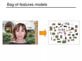
23. Bag-of-features for image classification • Origin: texture recognition • Texture is characterized by the repetition of basic elements or textons Julesz, 1981; Cula & Dana, 2001; Leung & Malik 2001; Mori, Belongie & Malik, 2001; Schmid 2001; Varma & Zisserman, 2002, 2003; Lazebnik, Schmid & Ponce, 2003

24. Texture recognition histogram Universal texton dictionary Julesz, 1981; Cula & Dana, 2001; Leung & Malik 2001; Mori, Belongie & Malik, 2001; Schmid 2001; Varma & Zisserman, 2002, 2003; Lazebnik, Schmid & Ponce, 2003

25. US Presidential Speeches Tag Cloudhttp://chir.ag/phernalia/preztags/ Bag-of-features for image classification • Origin: bag-of-words • Orderless document representation: frequencies of words from a dictionary • Classification to determine document categories

26. Bag-of-features for image classification SVM Extract regions Compute descriptors Find clusters and frequencies Compute distance matrix Classification [Nowak,Jurie&Triggs,ECCV’06], [Zhang,Marszalek,Lazebnik&Schmid,IJCV’07]

27. Bag-of-features for image classification SVM Extract regions Compute descriptors Find clusters and frequencies Compute distance matrix Classification Step 1 Step 3 Step 2 [Nowak,Jurie&Triggs,ECCV’06], [Zhang,Marszalek,Lazebnik&Schmid,IJCV’07]

28. bikes books building cars people phones trees Bag-of-features for image classification • Excellent results in the presence of background clutter

29. Examples for misclassified images Books- misclassified into faces, faces, buildings Buildings- misclassified into faces, trees, trees Cars- misclassified into buildings, phones, phones

30. Step 1: feature extraction • Scale-invariant image regions + SIFT (see lecture 2) • Affine invariant regions give “too” much invariance • Rotation invariance in many cases “too” much invariance • Dense descriptors • Improve results in the context of categories (for most categories) • Interest points do not necessarily capture “all” features

31. Dense features - Multi-scale dense grid: extraction of small overlapping patches at multiple scales - Computation of the SIFT descriptor for each grid cells

32. Step 1: feature extraction • Scale-invariant image regions + SIFT (see lecture 2) • Affine invariant regions give “too” much invariance • Rotation invariance for many realistic collections “too” much invariance • Dense descriptors • Improve results in the context of categories (for most categories) • Interest points do not necessarily capture “all” features • Color-based descriptors • Shape-based descriptors

33. … Step 2: Quantization

34. Step 2:Quantization Clustering

35. Step 2: Quantization Visual vocabulary Clustering

36. Examples for visual words

37. Step 2: Quantization • Cluster descriptors • K-mean • Gaussian mixture model • Assign each visual word to a cluster • Hard or soft assignment • Build frequency histogram

39. K-means clustering • We want to minimize sum of squared Euclidean distances between points xi and their nearest cluster centers Algorithm: • Randomly initialize K cluster centers • Iterate until convergence: • Assign each data point to the nearest center • Recompute each cluster center as the mean of all points assigned to it

41. K-means clustering • Local minimum, solution dependent on initialization • Initialization important, run several times • Select best solution, min cost

42. From clustering to vector quantization • Clustering is a common method for learning a visual vocabulary or codebook • Unsupervised learning process • Each cluster center produced by k-means becomes a codevector • Codebook can be learned on separate training set • Provided the training set is sufficiently representative, the codebook will be “universal” • The codebook is used for quantizing features • A vector quantizer takes a feature vector and maps it to the index of the nearest codevector in a codebook • Codebook = visual vocabulary • Codevector = visual word

43. Visual vocabularies: Issues • How to choose vocabulary size? • Too small: visual words not representative of all patches • Too large: quantization artifacts, overfitting • Computational efficiency • Vocabulary trees (Nister & Stewenius, 2006) • Soft quantization: Gaussian mixture instead of k-means

44. Gaussian mixture model (GMM) Gaussian density

45. Gaussian mixture model

48. Hard or soft assignment • K-means  hard assignment • Assign to the closest cluster center • Count number of descriptors assigned to a center • Gaussian mixture model  soft assignment • Estimate distance to all centers • Sum over number of descriptors • Frequency histogram

49. ….. Image representation frequency codewords