Download

1 / 25
250 likes | 540 Views
The Assumptions of ANOVA. Dennis Monday Gary Klein Sunmi Lee May 10, 2005. Major Assumptions of Analysis of Variance . The Assumptions Independence Normally distributed Homogeneity of variances Our Purpose Examine these assumptions Provide various tests for these assumptions Theory

E N D
The Assumptions of ANOVA Dennis Monday Gary Klein Sunmi Lee May 10, 2005
Major Assumptions of Analysis of Variance • The Assumptions • Independence • Normally distributed • Homogeneity of variances • Our Purpose • Examine these assumptions • Provide various tests for these assumptions • Theory • Sample SAS code (SAS, Version 8.2) • Consequences when these assumptions are not met • Remedial measures
Normality • Why normal? • ANOVA is anAnalysis of Variance • Analysis of two variances, more specifically, the ratio of two variances • Statistical inference is based on the F distribution which is given by the ratio of two chi-squared distributions • No surprise that each variance in the ANOVA ratio come from a parent normal distribution • Calculations can always be derived no matter what the distribution is. Calculations are algebraic properties separating sums of squares. Normality is only needed for statistical inference.
NormalityTests • Wide variety of tests we can perform to test if the data follows a normal distribution. • Mardia (1980) provides an extensive list for both the univariate and multivariate cases, categorizing them into two types • Properties of normal distribution, more specifically, the first four moments of the normal distribution • Shapiro-Wilk’s W (compares the ratio of the standard deviation to the variance multiplied by a constant to one) • Goodness-of-fit tests, • Kolmogorov-Smirnov D • Cramer-von Mises W2 • Anderson-Darling A2
NormalityTests procunivariate data=temp normal plot; var expvar; run; procunivariate data=temp normal plot; var normvar; run; Tests for Normality Test --Statistic--- -----p Value------ Shapiro-Wilk W 0.731203 Pr < W <0.0001 Kolmogorov-Smirnov D 0.206069 Pr > D <0.0100 Cramer-von Mises W-Sq 1.391667 Pr > W-Sq <0.0050 Anderson-Darling A-Sq 7.797847 Pr > A-Sq <0.0050 Tests for Normality Test --Statistic--- -----p Value------ Shapiro-Wilk W 0.989846 Pr < W 0.6521 Kolmogorov-Smirnov D 0.057951 Pr > D >0.1500 Cramer-von Mises W-Sq 0.03225 Pr > W-Sq >0.2500 Anderson-Darling A-Sq 0.224264 Pr > A-Sq >0.2500 Stem Leaf # Boxplot 22 1 1 | 20 7 1 | 18 90 2 | 16 047 3 | 14 6779 4 | 12 469002 6 | 10 2368 4 | 8 005546 6 +-----+ 6 228880077 9 | | 4 5233446 7 | | 2 3458447 7 *-----* 0 366904459 9 | + | -0 52871 5 | | -2 884318651 9 | | -4 98619 5 +-----+ -6 60 2 | -8 98557220 8 | -10 963 3 | -12 584 3 | -14 853 3 | -16 0 1 | -18 4 1 | -20 8 1 | ----+----+----+----+ Multiply Stem.Leaf by 10**-1 Normal Probability Plot 8.25+ | * | | | * | | * | + 4.25+ ** ++++ | ** +++ | *+++ | +++* | ++**** | ++++ ** | ++++***** | ++****** 0.25+* * ****************** +----+----+----+----+----+----+----+----+----+----+ Normal Probability Plot 2.3+ ++ * | ++* | +** | +** | **** | *** | **+ | ** | *** | **+ | *** 0.1+ *** | ** | *** | *** | ** | +*** | +** | +** | **** | ++ | +* -2.1+*++ +----+----+----+----+----+----+----+----+----+----+ -2 -1 0 +1 +2 Stem Leaf # Boxplot 8 0 1 * 7 7 6 6 1 1 * 5 5 2 1 * 4 5 1 0 4 4 1 0 3 588 3 0 3 3 1 0 2 59 2 | 2 00112234 8 | 1 56688 5 | 1 00011122223444 14 +--+--+ 0 55555566667777778999999 23 *-----* 0 000011111111111112222222233333334444444 39 +-----+ ----+----+----+----+----+----+----+----
Consequences of Non-Normality • F-test is very robust against non-normal data, especially in a fixed-effects model • Large sample size will approximate normality by Central Limit Theorem (recommended sample size > 50) • Simulations have shown unequal sample sizes between treatment groups magnify any departure from normality • A large deviation from normality leads to hypothesis test conclusions that are too liberal and a decrease in power and efficiency
Remedial Measures for Non-Normality • Data transformation • Be aware - transformations may lead to a fundamental change in the relationship between the dependent and the independent variable and is not always recommended. • Don’t use the standard F-test. • Modified F-tests • Adjust the degrees of freedom • Rank F-test (capitalizes the F-tests robustness) • Randomization test on the F-ratio • Other non-parametric test if distribution is unknown • Make up our own test using a likelihood ratio if distribution is known
Independence • Independent observations • No correlation between error terms • No correlation between independent variables and error • Positively correlated data inflates standard error • The estimation of the treatment means are more accurate than the standard error shows.
Independence Tests • If we have some notion of how the data was collected, we can check if there exists any autocorrelation. • The Durbin-Watson statistic looks at the correlation of each value and the value before it • Data must be sorted in correct order for meaningful results • For example, samples collected at the same time would be ordered by time if we suspect results could depend on time
Independence Tests procglm data=temp; class trt; model y = trt / p; output out=out_ds r=resid_var; run; quit; data out_ds; set out_ds; time = _n_; run; procgplot data=out_ds; plot resid_var * time; run; quit; procglm data=temp; class trt; model y = trt / p; output out=out_ds r=resid_var; run; quit; data out_ds; set out_ds; time = _n_; run; procgplot data=out_ds; plot resid_var * time; run; quit; First Order Autocorrelation 0.00479029 Durbin-Watson D 1.96904290 First Order Autocorrelation 0.90931 Durbin-Watson D 0.12405
Remedial Measures for Dependent Data • First defense against dependent data is proper study design and randomization • Designs could be implemented that takes correlation into account, e.g., crossover design • Look for environmental factors unaccounted for • Add covariates to the model if they are causing correlation, e.g., quantified learning curves • If no underlying factors can be found attributed to the autocorrelation • Use a different model, e.g., random effects model • Transform the independent variables using the correlation coefficient
Homogeneity of Variances • Eisenhart (1947) describes the problem of unequal variances as follows • the ANOVA model is based on the proportion of the mean squares of the factors and the residual mean squares • The residual mean square is the unbiased estimator of 2, the variance of a single observation • The between treatment mean squares takes into account not only the differences between observations, 2,just like the residual mean squares, but also the variance between treatments • If there was non-constant variance among treatments, we can replace the residual mean square with some overall variance, a2, and a treatment variance, t2, which is some weighted version of a2 • The “neatness” of ANOVA is lost
Homogeneity of Variances • The omnibus (overall) F-test is very robust against heterogeneity of variances, especially with fixed effects and equal sample sizes. • Tests for treatment differences like t-tests and contrasts are severely affected, resulting in inferences that may be too liberal or conservative.
Tests for Homogeneity of Variances • Levene’s Test • computes a one-way-anova on the absolute value (or sometimes the square) of the residuals, |yij – ŷi| with t-1, N – t degrees of freedom • Considered robust to departures of normality, but too conservative • Brown-Forsythe Test • a slight modification of Levene’s test, where the median is substituted for the mean (Kuehl (2000) refers to it as the Levene (med) Test) • The Fmax Test • Proportion of the largest variance of the treatment groups to the smallest and compares it to a critical value table • Tabachnik and Fidell (2001) use the Fmax ratio more as a rule of thumb rather than using a table of critical values. • Fmax ratio is no greater than 10 • Sample sizes of groups are approximately equal (ratio of smallest to largest is no greater than 4) • No matter how the Fmax test is used, normality must be assumed.
Tests for Homogeneity of Variances procglm data=temp; class trt; model y = trt; means trt / hovtest=levene hovtest=bf; run; quit; procglm data=temp; class trt; model y = trt; means trt / hovtest=levene hovtest=bf; run; quit; Homogeneous Variances The GLM Procedure Levene's Test for Homogeneity of Y Variance ANOVA of Squared Deviations from Group Means Sum of Mean Source DF Squares Square F Value Pr > F TRT 1 10.2533 10.2533 0.60 0.4389 Error 98 1663.5 16.9747 Brown and Forsythe's Test for Homogeneity of Y Variance ANOVA of Absolute Deviations from Group Medians Sum of Mean Source DF Squares Square F Value Pr > F TRT 1 0.7087 0.7087 0.56 0.4570 Error 98 124.6 1.2710 Heterogenous Variances The GLM Procedure Levene's Test for Homogeneity of y Variance ANOVA of Squared Deviations from Group Means Sum of Mean Source DF Squares Square F Value Pr > F trt 1 10459.1 10459.1 36.71 <.0001 Error 98 27921.5 284.9 Brown and Forsythe's Test for Homogeneity of y Variance ANOVA of Absolute Deviations from Group Medians Sum of Mean Source DF Squares Square F Value Pr > F trt 1 318.3 318.3 93.45 <.0001 Error 98 333.8 3.4065
Tests for Homogeneity of Variances • SAS (as far as I know) does not have a procedure to obtain Fmax (but easy to calculate) • More importantly: VARIANCE TESTS ARE ONLY FOR ONE-WAY ANOVA WARNING: Homogeneity of variance testing and Welch's ANOVA are only available for unweighted one-way models.
Tests for Homogeneity of Variances(Randomized Complete Block Design and/or Factorial Design) • In a CRD, the variance of each treatment group is checked for homogeneity • In factorial/RCBD, each cell’s variance should be checked H0: σij2 = σi’j’2, For all i,j where i ≠ i’, j ≠ j’
Tests for Homogeneity of Variances(Randomized Complete Block Design and/or Factorial Design) • Approach 1 • Code each row/column to its own group • Run HOVTESTS as before • Approach 2 • Recall Levene’s Test and Brown-Forsythe Test are ANOVAs based on residuals • Find residual for each observation • Run ANOVA data newgroup; set oldgroup; if block = 1 and treat = 1 then newgroup = 1; if block = 1 and treat = 2 then newgroup = 2; if block = 2 and treat = 1 then newgroup = 3; if block = 2 and treat = 2 then newgroup = 4; if block = 3 and treat = 1 then newgroup = 5; if block = 3 and treat = 2 then newgroup = 6; run; procglm data=newgroup; class newgroup; model y = newgroup; means newgroup / hovtest=levene hovtest=bf; run; quit; procsort data=oldgroup; by treat block; run; procmeans data=oldgroup noprint; by treat block; var y; output out=stats mean=mean median=median; run; data newgroup; merge oldgroup stats; by treat block; resid = abs(mean - y); if block = 1 and treat = 1 then newgroup = 1; ……… run; procglm data=newgroup; class newgroup; model resid = newgroup; run; quit;
Tests for Homogeneity of Variances(Repeated-Measures Design) • Recall the repeated-measures set-up:
Tests for Homogeneity of Variances(Repeated-Measures Design) • As there is only one score per cell, the variance of each cell cannot be computed. Instead, four assumptions need to be tested/satisfied • Compound Symmetry • Homogeneity of variance in each column • σa12 = σa22 =σa32 • Homogeneity of covariance between columns • σa1a2=σa2a3= σa3a1 • No A x S Interaction (Additivity) • Sphericity • Variance of difference scores between pairs are equal • σYa1-Ya2= σYa1-Ya3= σYa2-Ya3
Tests for Homogeneity of Variances(Repeated-Measures Design) • Usually, testing sphericity will suffice • Sphericity can be tested using the Mauchly test in SAS procglm data=temp; class sub; model a1 a2 a3 = sub / nouni; repeated as 3 (123) polynomial / summary printe; run; quit; Sphericity Tests Mauchly's Variables DF Criterion Chi-Square Pr > ChiSq Transformed Variates 2 Det = 0 6.01 .056 Orthogonal Components 2 Det = 0 6.03 .062
Tests for Homogeneity of Variances(Latin-Squares/Split-Plot Design) • If there is only one score per cell, homogeneity of variances needs to be shown for the marginals of each column and each row • Each factor for a latin-square • Whole plots and subplots for split-plot • If there are repititions, homogeneity is to be shown within each cell like RCBD • If there are repeated-measures, follow guidelines for sphericity, compound symmetry and additivity as well
Remedial Measures for Heterogeneous Variances • Studies that do not involve repeated measures • If normality is not violated, a weighted ANOVA is suggested (e.g., Welch’s ANOVA) • If normality is violated, the data transformation necessary to normalize data will usually stabilize variances as well • If variances are still not homogeneous, non-ANOVA tests might be your option • Studies with repeated measures • For violations of sphericity • modify the degrees of freedom have been suggested. • Greenhouse-Geisser • Huynh and Feldt • Only do specific comparisons (sphericity does not apply since only two groups – sphericity implies more than two) • MANOVA • Use an MLE procedure to specify variance-covariance matrix
Other Concerns • Outliers and influential points • Data should always be checked for influential points that might bias statistical inference • Use scatterplots of residuals • Statistical tests using regression to detect outliers • DFBETAS • Cook’s D
References • Casella, G. and Berger, R. (2002). Statistical Inference. United States: Duxbury. • Cochran, W. G. (1947). Some Consequences When the Assumptions for the Analysis of Variances are not Satisfied. Biometrics. Vol. 3, 22-38. • Eisenhart, C. (1947). The Assumptions Underlying the Analysis of Variance. Biometrics. Vol. 3, 1-21. • Ito, P. K. (1980). Robustness of ANOVA and MANOVA Test Procedures. Handbook of Statistics 1: Analysis of Variance (P. R. Krishnaiah, ed.), 199-236. Amsterdam: North-Holland. • Kaskey, G., et al. (1980). Transformations to Normality. Handbook of Statistics 1: Analysis of Variance (P. R. Krishnaiah, ed.), 321-341. Amsterdam: North-Holland. • Kuehl, R. (2000). Design of Experiments: Statistical Principles of Research Design and Analysis, 2nd edition. United States: Duxbury. • Kutner, M. H., et al. (2005). Applied Linear Statistical Models, 5th edition. New York: McGraw-Hill. • Mardia, K. V. (1980). Tests of Univariate and Multivariate Normality. Handbook of Statistics 1: Analysis of Variance (P. R. Krishnaiah, ed.), 279-320. Amsterdam: North-Holland. • Tabachnik, B. and Fidell, L. (2001). Computer-Assisted Research Design and Analysis. Boston: Allyn & Bacon.