Download
1 / 7
80 likes | 172 Views
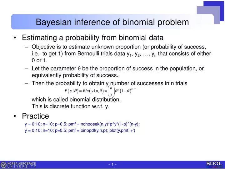
Bayesian inference of binomial problem. Estimating a probability from binomial data Objective is to estimate unknown proportion (or probability of success, i.e., to get 1) from Bernoulli trials data y 1 , y 2 , …, y n that consists of either 0 or 1.

E N D
Bayesian inference of binomial problem • Estimating a probability from binomial data • Objective is to estimate unknown proportion (or probability of success, i.e., to get 1) from Bernoulli trials data y1, y2, …, yn that consists of either 0 or 1. • Let the parameter q be the proportion of success in the population, or equivalently probability of success. • Then the probability to obtain y number of successes in n trials which is called binomial distribution.This is discrete function w.r.t. y. • Practice y = 0:10; n=10; p=0.5; pmf = nchoosek(n,y)*p^y*(1-p)^(n-y); y = 0:10; n=10; p=0.5; pmf = binopdf(y,n,p); plot(y,pmf,'+')
Bayesian inference of binomial problem • Inference problem statement • Let the parameter q be the proportion of females in the population. • Current accepted value in Europe is 0.485, less than 0.5. • Estimate q conditional on the observed data: y females out of n births. • Simplest way is just to let q = y/n. • Bayesian inference • Assume non-informative prior: q ~ uniform on [0, 1]. • Likelihood: • Posterior density:
Bayesian inference of binomial problem • Illustrative results • Several different experiments but with same proportion of successeswhere sample sizes vary. • Interpret the meaning of the figures. • Practice: plot the four cases using matlab function.
Bayesian inference of binomial problem • Beta pdf • In fact, the posterior density is beta distribution with parameters a = y+1, b = n-y+1. • Practice : plot the four cases using beta pdf function. • Laplace in 18th Century • 241,945 girls, 251,527 boys in Paris during 1745 ~ 1770. • P[q ≥ 0.5 | y] ≈ 1.1510-42 So he was ‘certain’ that q < 0.5. • Practice: calculate this value, and validate. • Posterior prediction • What is the probability to get girl if a new baby born ? • Practice: calculate this value. What if the numbers were 2 out of 5 ?
Bayesian inference of binomial problem • Summarizing posterior inference • Locations summary: • Mean: expectation, needs integration. • Mode: most-likely value. Maximum of pdf. Needs optimization or d(pdf)/dx. • Median: 50% percentile value. • Among these, mode is preferred due to the computational convenience. • Variations summary: • Standard deviation or variance • Interquartile range or 100(1-a)% interval • Practice with beta pdf.Mean, mode are given as equation analytically.Others are obtained using matlab functions. • In general, these values are computed using computer simulations from the posterior distribution.
Bayesian inference of binomial problem • Informative prior • So far considered only uniform prior. • Recall the likelihood is binomial pdf: • Let us introduce prior of beta pdf: where a, b are called hyperparameters. • Then posterior density: • Remarks • Property that posterior distribution follows same form as the prior is called conjugacy. Beta prior is conjugate family of binomial likelihood. • As a result, the mean & variance of posterior pdf: • As y & n-y become large under fixed a & b,In the limit, parameters of the prior have no influence on posterior.Besides, it converges to normal pdf due to central limit theorem.
Homework • 2.5 example: estimating probability of female birth • P[ q < 0.485 ] • Histogram of posterior pdfq|y • Median and 95% confidence intervals. Ans .446, [.415, .477]