Download
1 / 26

E N D
Introduction Huffman codes are a very effective technique for compressing data; savings of 20% to 90% are typical, depending on the characteristics of the file being compressed. Huffman’s greedy algorithm uses a table of frequencies of occurrence of each character in the file to build up an optimal way of representing each character as a binary string. Suppose we have a 100,000-character data file that we wish to store compactly. Further suppose the characters in the file occur with the following frequencies:
Introduction That is, there are only 6 different characters in the file, and, for example, the character aappears 45,000 times. There are many ways to represent such a file of information. We consider the problem of designing a binary character code (or code for short), wherein each character is represented by a unique binary string. If we use a fixed-length code, we need 3 bits to represent six characters, and 300,000 bits for the entire file.
Introduction A variable-length code can do considerably better, by giving frequent characters short codewords, and infrequent characters long codewords. In our example: If we use the given variable-length code, we only need 224,000 bits (1*45+3*13+3*12+3*16+4*9+4*5=224). We saved approximately 25%. In fact, this is an optimal character code for this file.
Prefix codes We consider here only codes in which no codeword is also a prefix of some other codeword. Such codes are are called prefix(-free) codes. Itispossible to show that optimal data compression achievable by a character code can always be achieved with a prefix code, so there is no loss of generality in restricting attention to prefix codes.
Prefix codes Prefix codes are desirable because they simplify encoding (compression) and decoding. Encoding is always easy for any binary character code; we just concatenate the codewords representing each character of the file. In the example, we code “abc” by 0101100 (if we use the variable-length prefix code).
Prefix codes Decoding is also quite simple with a prefix code. Since no codeword is a prefix of any other, the codeword that begins an encoded file is unambiguous. We can simply identify the initial codeword, translate it back to the original character, remove it from the encoded file, and repeat the decoding process on the remainder of the encoded file. In our example, the string 001011101 parses uniquely as 0 0 101 1101, which decodes to “aabe”.
Prefix codes The decoding process needs a convenient representation for the prefix code so that the initial codeword can be easily picked off. A binary tree whose leaves are the given characters provides one such representation. We interpret the binary codeword for a character as the path form the root to the character, where 0 means “go to the left child” and 1 means “go to the right child”. The following figure shows the trees for the two codes of our example.
Prefix codes An optimal code for a file is always represented by a full binary tree, in which every nonleaf node has two children (why?). The fixed-length code in our example is not optimal since its tree is not a full binary tree: there are codewords beginning 10…, but none beginning 11…. Since we can now restrict our attention to full binary trees, we can say that if C is the alphabet from which the characters are drawn, then the tree for an optimal prefix code has exactly |C| leaves, one for each letter of the alphabet, and exactly |C| -1 internal nodes.
Prefix codes Given a tree T corresponding to a prefix code, it is a simple matter to compute the number of bits required to encode a file. For each character c in the alphabet C, let f(c) denote the frequency of c in the file and let dT(c) denote the depth of c’s leaf in the tree. Note that dT(c) is also the length of the codeword for the character c. The number of bits required to encode a file is thus B(T) = ∑cC f(c) dT(c) Which is defined as the cost of the tree T.
Constructing a Huffman code Huffman invented a greedy algorithm that constructs an optimal prefix code called a Huffman code. In the pseudocode that follows, C is a set of n characters and each cC has a defined frequency f[c].The algorithm builds the tree T corresponding to the optimal code in a bottom-up manner. It begins with a set of |C| leaves and performs a sequence of |C| -1 “merging” operations to create the final tree. A priority queue Q, keyed on f, is used to identify the two least-frequent objects to merge together. The result of the merger of two objects is the a new object whose frequency is the sum of the frequencies of the two objects that were merged.
Constructing a Huffman code HUFFMAN(C) n |C| Q C fori 1 to n-1 do allocate a new node z left[z] x EXTRACT-MIN(Q) right[z] y EXTRACT-MIN(Q) f[z] f[x] + f[y] INSERT(Q,z) return EXTRACT-MIN(Q)
Constructing a Huffman code For our example, the following figures show how the algorithm works. There are 6 letters, and so the size of the initial queue is n = 6. There are 5 merge steps. The final tree represents the optimal prefix code. The codeword for a letter is a sequence of the edge labels on the path from the root to the letter.
Constructing a Huffman code The analysis of the code is quite simple: we first define the queue, then we have n-1 merge steps: we pick the two most infrequent characters and merge them to a new one, that finds its proper place in the queue. If we implement the queue via a heap, the running time is easily found to be O(nlog n).
Correctness of Huffman’s algorithm We present several lemmas that will lead to the desired conclusion. Lemma 16.2: Let C be an alphabet in which each character cC has frequency f[c]. Let x and y be two characters in C having the lowest frequencies. Then there exists an optimal prefix code for C in which thecodewords for x and y have the same length and differ only in the last bit.
Correctness of Huffman’s algorithm Proof: The idea is to take the tree T representing an arbitrary optimal prefix code and modify it to make a tree representing another optimal prefix code such that the characters x and y appear as sibling leaves of maximum depth in the new tree. If we succeed, then their codewords will have the same length and will only differ in the last bit.
Correctness of Huffman’s algorithm Let a and b be two characters that are sibling leaves of maximum depth in T. Without loss of generality, we assume that f[a] f[b] and f[x] f[y]. Since f[x] and f[y] are the two lowest leaf frequencies, in order, and f[a] and f[b] are two arbitrary frequencies, in order, we have f[x] f[a], and f[y] f[b]. We now exchange the positions in T of a and x, and get the tree T’, and then exchange the positions of b and y, to produce the tree T’’. We should now calculate the difference in cost between T and T’’.
Correctness of Huffman’s algorithm We start with B(T) - B(T’) = ∑cC f[c] dT(c) - ∑cC f[c] dT’(c) = f[x] dT(x) + f[a] dT(a) - f[x] dT’(x) - f[a] dT’(a) = f[x] dT(x) + f[a] dT(a) - f[x] dT(a) - f[a] dT(x) = ( f[a] - f[x] ) ( dT(a) - dT(x) ) 0, because both f[a] - f[x] and dT(a) - dT(x) are nonnegative (Why?). Similarly, when we move from T’ to T’’, we do not increase the cost. Therefore, B(T’’) B(T), but since T was optimal, B(T) B(T’’), which implies B(T) = B(T’’). Thus, T’’ is an optimal tree in which x and y appear as sibling leaves of maximum depth, and the lemma follows.
Correctness of Huffman’s algorithm The lemma implies that the process of building up an optimal tree by mergers can, without loss of generality, begin with the greedy choice of merging together two characters of lowest frequency. The next lemma shows that the problem of constructing optimal prefix codes has (what we call) the optimal substructure property:
Correctness of Huffman’s algorithm Lemma 16.3: Let T be a full binary tree representing an optimal prefix code over an alphabet C, wherefrequency f[c]isdefinedforeachcharacter cC. Consider any two characters x and y that appear as sibling leaves in T, and let z be their parent. Then, considering z as a character with frequency f[z] = f[x] + f[y], the tree T’ = T – { x, y } represents an optimal prefix code for the alphabet C’ = C –{ x, y } { z }.
Correctness of Huffman’s algorithm Proof: We first show that the cost B(T) of the tree T can be expressed in terms of the cost B(T’) of the tree T’ by considering the different summands in the definition of B( ). For each c C –{ x, y }, we have dT(c) = dT’(c), resulting in f[c] dT(c) = f[c] dT’(c). Since dT(x) = dT(y) = dT’(z) + 1, we have f[x] dT(x) + f[y] dT(y) = ( f[x] + f[y]( ( dT’(z) + 1 ) = f[z] dT’(z) + ( f[x] + f[y](, leading to B(T) = B(T’) + f[x] + f[y].
Correctness of Huffman’s algorithm If T’ represents a non-optimal prefix code for the alphabet C’, then there exists atree T’’ whose leave are characters in C’ such that B(T’’) < B(T’). Since z is treated as a character in C’, it appears as a leaf in T’’. If we add x and y as the children of z in T’’, we obtain a prefix code for C with cost B(T’’) + f[x] + f[y] < B(T), contradicting the optimality of T. Thus, T’ must be optimal for the alphabet C’.
Correctness of Huffman’s algorithm Theorem: Procedure HUFFMANproduces an optimal prefix code. Proof: Immediate from the two lemmas. Last updated: 2/08/2010