Download
1 / 26
390 likes | 930 Views
Manifold learning. Jan Kamenický. Nonlinear dimensionality reduction. Many features ⇒ many dimensions Dimensionality reduction Feature extraction (useful representation) Classification Visualization. Manifold learning. WhaT maniFold ?

E N D
Manifold learning Jan Kamenický
Nonlinear dimensionality reduction • Many features ⇒ many dimensions • Dimensionality reduction • Feature extraction (useful representation) • Classification • Visualization
Manifold learning • WhaTmaniFold? • Low dimensional embedding of high dimensional data lying on a smooth nonlinear manifold • Linear methods fail • i.e. PCA
Manifold learning • Unsupervised methods • Without any a priori knowledge • ISOMAPs • Isometric mapping • LLE • Locally linear embedding
ISOMAP • Core idea • Use geodesic distances on the manifold instead of Euclidean • Classical MDS • Maps data to the lower dimensional space
Estimating geodesic distances • Select neighbours • K-nearest neighbours • ε-distance neighbourhood • Create weighted neighbourhood graph • Weights = Euclidean distances • Estimate the geodesic distancesas shortest paths in the weighted graph • Dijkstra’s algorithm
Dijkstra’s algorithm • 1) Set distances (0 for initial, ∞ for all other nodes), set all nodes as unvisited • 2) Select unvisited node with smallest distance as active • 3) Update all unvisited neighbours of the active node (if the computed distance is smaller) • 4) Mark active node as visited (it has now minimal distance), repeat from 2) as necessary
Dijkstra’s algorithm • Time complexity • O(|E|dec+|V|min) • Implementation • Sparse edges • Fibonacci heap as a priority queue • O(|E|+|V|log|V|) • Geodesic distances in ISOMAP • O(N2logN)
Multidimensional scaling (MDS) • Input • Dissimilarities (distances) • Output • Data in a low-dimensional embedding, with distances corresponding to the dissimilarities • Many types of MDS • Classical • Metric / non-metric (number of dissimilarity matrices, symmetry, etc.)
Classical MDS • Quantitative similarity • Euclidean distances (output) • One distance matrix (symmetric) • Minimizing the stress function
Classical MDS • We can optimize directly • Compute double-centered distance matrix • Note: • Perform SVD of B • Compute final data
MDS and PCA correspondence • Covariance matrix • Projection of centered X onto eigenvectors of NS (result of the PCA of X)
ISOMAP • How many dimensions to use? • Residual variance • Short-circuiting • Too large neigbourhood (not enough data) • Non-isometric mapping • Totally destroys the final embedding
ISOMAP modifications • Conformal ISOMAP • Modified weights in geodesic distance estimate: • Magnifies regions with high density • Shrinks regions with low density
ISOMAP modifications • Landmark ISOMAP • Use only geodesic distances from several landmark points (on the manifold) • Use Landmark-MDS for finding the embedding • Involves triangulation of non-landmark data • Significantly faster, but higher chance for “short-circuiting”, number of landmarks has to be chosen carefully
ISOMAP modifications • Kernel ISOMAP • Ensures that the B (double-centered distance matrix) is positive semidefinite by constant-shifting method
Locally linear embedding • Core idea • Estimate each point as a linear combination of it’s neighbours – find best such weights • Same linear representation will hold in the low dimensional space
LLE • Find weights Wij by constrained minimization • Neighbourhood preserving mapping
LLE • Low dimensional representation Y • We take eigenvectors of M corresponding to its q+1 smallest eigenvalues • Actually, different algebra is used to improve numeric stability and speed
ISOMAP vs LLE • ISOMAP • Preserves global geometric properties (geodesic distances), especially for faraway points • LLE • Preserves local neighbourhood correspondence only • Overcomes non-isometric mapping • Manifold is not explicitly required • Difficult to estimate q (number of dimensions)