Download
1 / 14
901 likes | 1.97k Views
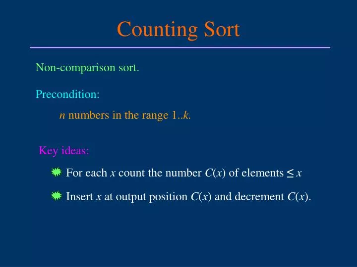
Counting Sort. Non-comparison sort. Precondition:. n numbers in the range 1.. k. Key ideas:. For each x count the number C ( x ) of elements ≤ x. Insert x at output position C ( x ) and decrement C ( x ). 1 2 3 4 5 6 7. 2. 2.

E N D
Counting Sort Non-comparison sort. Precondition: n numbers in the range 1..k. Key ideas: For each x count the number C(x) of elements ≤ x Insert x at output position C(x) and decrement C(x).
1 2 3 4 5 6 7 2 2 2 2 1 0 2 Auxiliary storage C[1..k] 1 2 3 4 5 6 7 2 4 6 8 9 9 11 C An Example 1 2 3 4 5 6 7 8 9 10 11 Input 7 1 3 1 2 4 5 7 2 4 3 A[1..n] k fori= 2 to 7 doC[i] =C[i] +C[i–1] two 1’s inA 6 elements ≤ 3
1 2 3 4 5 6 7 8 9 10 11 Output B[1..n] 1 2 3 4 5 6 7 C 2 4 6 8 9 9 11 1 2 3 4 5 6 7 2 4 5 8 9 9 11 C Example (continued) A[1..n] 3 B[6] =B[C[3]] =B[C[A[11]]] =A[11] = 3 C[A[11]] =C[A[11]] – 1
1 2 3 4 5 6 7 2 4 5 7 9 9 11 C Example (cont’d) 1 2 3 4 5 6 7 8 9 10 11 3 4 B B[C[A[10]]] =A[10] = 4 1 2 3 4 5 6 7 C 2 4 5 8 9 9 11 C[A[10]] =C[A[10]]– 1
Example (cont’d) 1 2 3 4 5 6 7 8 9 10 11 2 3 4 4 5 7 B B[C[A[6]]] =A[6] = 4 1 2 3 4 5 6 7 C 2 3 5 7 8 9 10 C[A[6]] =C[A[6]] – 1 1 2 3 4 5 6 7 2 3 5 6 8 9 10 C
Analysis of Counting Sort Counting-Sort(A, B, k) for i = 1 tok doC[i] = 0 // (k) for j= 1 to length[A] doC[A[j]] =C[A[j]] + 1//(n) //C[i] now contains the number of elements =i fori= 2 tok doC[i] =C[i] +C[i–1]//(k) //C[i] now contains the number of elements ≤i for j = length[A] downto 1 doB[C[A[j]]] =A[j] C[A[j]] =C[A[j]] – 1// (n) Running time is(n+k)(or(n)if k = O(n))!
Stability Counting sort isstable: Input order maintained among items with equal keys. Stability is important because data are often carried with the keys being sorted. radix sort (which uses counting sort as a subroutine) relies on it to work correctly. How is stability realized? forj = length[A] downto 1 doB[C[A[j]]] =A[j] C[A[j]] =C[A[j]] – 1
Pass 1: Radix Sort Sort a set of numbers in multiplepasses, starting from the rightmost digit, then the 10’s digit, then the 100’s digit, etc. Example: sort 23, 45, 7, 56, 20, 19, 88, 77, 61, 13, 52, 39, 80, 2, 99 99 77 80 2 13 39 7 88 20 61 52 23 45 56 19 Pass 2: 88 7 23 56 19 61 77 80 99 20 52 2 13 39 45
Analysis of Radix Sort Correctnessfollows by induction on the number of passes. Sort n d-digit numbers. Let k be the range of each digit. Each pass takes time (n+k).// use counting sort There are d passes in total. The running time for radix sort is(dn+dk). Linear running timewhen d is a constant and k = O(n).
r Each digit in the range 0 -- 2 – 1 r b/r passes, each spending time (n+2 ). r Running time((b/r) (n + 2 )). If b≤ lg n, choose r= b(n) If b> lg n, choose r= lg n(bn/lg n) Breaking into Digits b bits Key: … … b/r digits r-bit digit
Bucket Sort Assumption: input elements are uniformly distributed over [0, 1) In case the input range is larger than 1, normalize each element over the maximum first. n buckets are used for n input numbers. Insert A[i] into bucket nA[i] , 1 in. Bucket sort runs in(n)expected time.
An Example A[ ] 0 .78 .17 1 .12 .17 2 .39 .21 .23 .26 3 .26 .39 4 .72 5 .94 6 .21 .68 .12 7 .72 .78 8 .23 9 .68 .94 n inputs dropped into n equal-sized subintervals of [0, 1). Step 2: Concatenate all lists Step 1: equivalent of insertion sort within each list
Bucket sort n +(n+100).0175n + 18n 3.5n 645 35246 2 2 Comparison of Sorting Methods (II) Method Space Average Max n=16 n=10000 Counting sort 2n + 1000 22n + 10010 22n 10362 32010 Radix sort n +(n+200) 32n 32n + 4838 4250 36838 D. E. Knuth, “The Art of Computer Programming”, Vol 3, 2nd ed., p.382, 1998. Implemented on the MIX Computer.
Comparison of Sorting Algorithms Insertion sort: suitable only for small n. Merge sort: guaranteed to be fast even in its worst case; stable. Heapsort: requiring minimum memory and guaranteed to run fast; average and maximum time both roughly twice the average time of quicksort. Quicksort: most useful general-purpose sorting for very little memory requirement and fastest average time. (choose the median of three elements as pivot in practice :-) Counting sort: very useful when the keys have small range; stable; memory space for counters and for 2n records. Radix sort: appropriate for keys either rather short or with a lexicographic collating sequence. Bucket sort: assuming keys to have uniform distribution.