Download
1 / 13
130 likes | 263 Views
Simulation of the Argo observing system. Igor Kamenkovich, RSMAS, University of Miami Wei Cheng, E.S. Sarachik and D.E.Harrison University of Washington. Introduction. The Argo system. Argo array has been brought to the full strength of 3000 floats

E N D
Simulation of the Argo observing system Igor Kamenkovich, RSMAS, University of Miami Wei Cheng, E.S. Sarachik and D.E.Harrison University of Washington
Introduction. The Argo system • Argo array has been brought to the full strength of 3000 floats • The floats reside at the depth of 1000-2000 meters, where they move with the flow • Every 10 days, the floats surface while taking vertical profiles of temperature and salinity • The density of global spatial coverage is unprecedented • Spatial resolution is still not sufficient for resolving sharp fronts and small-scale anomalies: average spacing between floats is ~ 300km • Advection of the floats by oceanic currents has a dual affect: • It increases spatial coverage • It shortens the time a float spends near any given location
float float d/2 d/2 U D Effects of advection Increase in spatial coverage: • What is the radius d/2 within which we are guaranteed to have a float within a time interval T? • This is the case if D-d < UT. If D is 300km and T is 1month d > D – UT ~ 300km if U = 1cm/sec ~ 50km if U = 10cm/sec • Most large-scale currents (except western boundary currents and ACC) are too weak to impact coverage; especially in the direction of sharp gradients • Strong advection by mesoscale eddies has a more pronounced effect
Effects of advection Decrease in time spent near a particular location: • Changes in float positions act to distort time dependency in sampled fields if UT is sufficiently large • For slow large-scale advection U ~ 1.0 - 0.1cm/sec, and the effects are noticeable only on long time scales (> 1 year) • Fast advection by eddies can noticeably redistribute floats within 1 month • Extreme case: random redistribution of floats every 10 days (upper bound on the effects of eddy advection): The probability that within a month, at least one float is within a radius 100km of a given location is about 30%
Observing System Simulation Experiments • The goal is to estimate the expected accuracy and limitations of the Argo observing system, by analyzing its simulations in ocean general circulation models (GCMs) (Arnold and Dey 1986) • Has been used for different observing systems (Kindle 1986; Barth and Wunsch 1990; Bennett 1990; Hernandez et al. 1995; Hackert et al. 1998) • For the Argo array, OSSEs concentrated on the Indian Ocean (Schiller et al. 2004; Oke and Schiller 2005; Ballabrera-Poy et al. 2007; Vecchi and Harrison 2007) and Mediterranean Sea (Griffa et al. 2006) • OSSE approach has several advantages: • the actual (GCM-simulated) field is known and thus the errors in the reconstructed fields can be accurately estimated • parameters of the observing system and the “observed” oceanic state can be modified in sensitivity studies • We use two GCMs: global coarse-resolution and regional eddy-resolving
Global coarse-resolution GCM Ocean model is based on the GFDL MOM with: • Global geometry; 2o 2o resolution; 25 vertical layers • Gent-McWilliams parameterization of mesoscale eddies • KPP boundary layer mixing scheme • Thermodynamic sea-ice model Forcing: • Surface fluxes calculated by bulk formulas • Daily wind stress, wind speed, and air temperature/humidity are taken from 23 years of NCEP reanalysis • At this resolution, GCM underestimates the intensity of fronts and western boundary currents • The “floats” reside at 1500m depth, surface every 10 days while taking measurements • T/S values are reconstructed on the original model grid using an OA method (Mariano and Brown 1992) • We analyze the reconstruction errors: the difference between the OA and actual GCM-simulated values
Errors in Upper Ocean Heat Content (UOHC) • UOHC is calculated over the top 800m, in a 5-year run • Annual means: errors are small, except within the western boundary currents and ACC • Amplitude of the annual cycle (Sep-March) in flux units: errors exceed 25-50 Wm-2 in some locations, but are generally small • Amplitude of the interannual trend (year 5 – year 1) in flux units: errors exceed 5-10 Wm-2 at high latitudes • Globally averaged error magnitude is 2.2 Wm-2
Errors in the Mixed layer Depth (MLD) • Very sensitive to T/S values; negative biases in T lead to the underestimated MLD • Annual means, amplitude of the annual cycle and magnitude of the interannual trend all exhibit: • Large errors in ACC (especially the Indian sector) • Large errors in the high-latitude North Atlantic
Sensitivity runs: Effects of float movements The “parked floats” case (float positions do not change in time): • Errors are larger in the standard run compare to the “parked floats” case • A large part of errors in the standard case is explained by advection The “random position” case (floats are redistributed randomly every 10 days): • Errors are reduced as a result of redistribution, due to the increased spatial coverage Difference in the magnitude of errors in the interannual trend between the standard and “parked floats” cases Difference in the magnitude of errors in the interannual trend between the “random position” and standard cases
Eddy-resolving North Atlantic model • Regional model of the North Atlantic: 14oN to 60oN • Eddy-resolving grid: 1/8o in latitude and longitude • 250 “floats” are released • 9-year run, no seasonal cycle • Mesoscale variability is the strongest in the subpolar gyre region • Reconstruction errors are the largest in the subpolar and Gulf Stream regions • Errors in SST and UOHC have similar structure • The errors increase even further when the mesoscale variability in the model is amplified (to match the observed intensity)
Eddy-resolving sensitivity runs • “Time-mean” case: mesoscale variability is removed by time-averaging • The errors are significantly reduced, in the subpolar gyre region • Are these eddy-induced errors due to the variability in advection or T/S fields? • “Mean advection” case: mesoscale variability is removed from the velocities only • Most of the eddy-induced errors are due to eddy advection, not T/S variability Difference in the magnitude of errors in the interannual trend between: (a) standard and time-mean; and (b) mean-advection and time-mean cases
Conclusions • Overall performance of the simulated Argo array is impressive • Global experiments, however, exhibit significant differences between the reconstructed and actual GCM-simulated fields within intense currents • The errors in the interannual trend are particularly significant compare to the actual signal • The advection has a dual effect on the reconstruction errors. Movement of the floats (i) increases the overall spatial coverage, but (ii) negatively impacts the ability to resolve time dependence • Large-scale advection negatively impacts the ability of the Argo system to reconstruct the magnitude of the annual cycle and interannual trend • Fast redistribution of floats increases the spatial coverage, which improves reconstruction of the interannual trend. These effects are similar to the effects of doubling the number of floats
Conclusions (cont.) • Explicitly simulated mesoscale eddies act to increase the reconstruction errors • These effects are mainly due to the strong, rapidly changing eddy velocities, rather than to the mesoscale variability in T/S Further directions: • Effects of mesoscale variability in ACC • Detection of realistic patterns of climate variability