Download
1 / 68
680 likes | 745 Views
International Economics: Trade Theory and Policy WS 2013/14 Christen/Leiter/Pfaffermayr Lecture: Mo. 8:30-11:00, HS3 Proseminar: see Syllabus. Literature van Marrewijk, Ch. (2012), International Economics, Oxford University Press, 2 nd ed. Chapters from Parts I, II and III

E N D
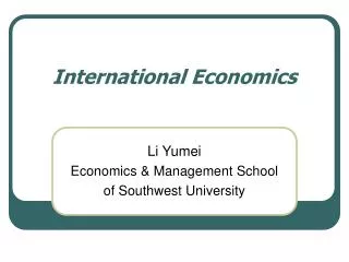
International Economics: Trade Theory and Policy WS 2013/14 Christen/Leiter/Pfaffermayr Lecture: Mo. 8:30-11:00, HS3 Proseminar: see Syllabus
Literature van Marrewijk, Ch. (2012), International Economics, Oxford University Press, 2nd ed. Chapters from Parts I, II and III Additional material will be covered in the Proseminar
Exam and Grading Includes all the material covered in the course (lecture plus proseminar). A positive grade in the PS is a necessity. Course grade is an ECTS-weighted average of exam and PS. An example of an exam plus some examples of exam questions are provided in OLAT. Three final exams per semester. Lecture: 70.0% Two short essays. You can choose from three topics. Proseminar: 30.0% Three short questions. .
Questions addressed in trade theory and policy I • Determinants of trade and industry structure of an open economy in the long run. • The welfare effects and distributional consequences (factor incomes) of worldwide globalization and trade liberalization. • Labor market effects of trade and foreign direct investment. • Trade Policy: Instruments and their welfare effectsThe impact and the welfare effects of regional trade agreements
Questions addressed in trade theory and policy II • Structural change and trade liberalization: Should European countries protect e.g. their textile industries? • ‘Are our wages set in Beijing?’: The impact of trade with low wage countries on low skilled workers’ wages in Europe. • Why do trade volumes grow faster than GDP? • What can we expect from the multilateral trade liberalization efforts of WTO? • The impact of a bilateral Trade Agreements, e.g., between EU and US?
Literature and Resources I • Study Guide: Stephan Schueller and Daniel Ottens Oxford University Press • Krugman, Paul R., Maurice Obstfeld and Marc J. Melitz: International Economics, Theory and Policy, Pearson, 9th ed., 2012. • Feenstra Robert C. and Alan M. Taylor, International Economics: International Edition, Worth Publishers, 2nd ed., 2011 • Further literature cited in these two books, especially papers in the academic journals
Literature and Resources II • FIW: http://www.fiw.ac.at/ • WIFO: http://www.wifo.ac.at/ • WIIW: http://www.wiiw.ac.at/ • WTO: http://www.wto.org/ • EU: http://ec.europa.eu/trade/ • WITS: http://wits.worldbank.org/wits/ • CEPII: http://www.cepii.fr/CEPII/en/bdd_modele/bdd.asp • UNCTAD: http://unctad.org/en/Pages/Statistics.aspx • GTAP: https://www.gtap.agecon.purdue.edu/ • Feeenstra: http://cid.econ.ucdavis.edu/data.html
Chapter 1: The World Economy – Some Stylized Facts p. 4: „International economics is what international economists do,…, you will only know about intern-ational economics, once you have studied it your-self“. „…I think that an important distinguishing cha-racteristic is the general equilibrium nature of this approach.“ This forces us to be precise and complete in our explanations.
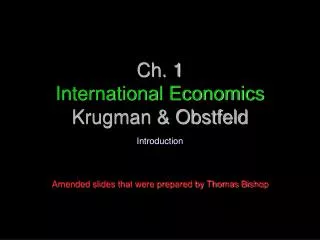
* The portrait was painted by Carla Rodenburg in 2001. I am grateful to Angus Maddison for his permission to use this painting. Angus Maddison Figure 1.1 Angus Maddison (1926 -2010)
Chap. 1.2 and 1.3: The economic size (power?) of a nation is best measured in terms of the total value of goods and services produced in a certain time period. Other measures of size such as land area and population are weakly correlated with economic size – look at Russia, China, India, Brazil on the one hand, and on the European Countries on the other hand.
A size comparison across open countries needs three steps: • Accurate data from the statistical offices in national currency (Maddison in our case). • Decide to look at GNP or GDP GDP + net receipts of factor income = GNP GDP…market value of goods and services produced by labor and property located in a country. GNP… market value of goods and services produced by labor and property of the nationals of a country. • Use the same currency ($): current US $ or PPP.
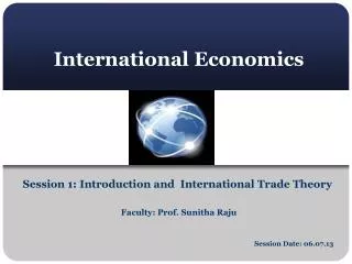
Fig 1.2: GDP and GNP, 2008 ($ billion) The dottedlineis a 45º line, theaxesuse a logarithmicscale, andthecirclesare proportional tothesizeof GDP.
Purchasing Power Parity (PPP) Comparing income in current $ tends to overestimatethe differences between high and low income countries (i) Tradable goods are subject to international competition so that the prices of such tradable goods tend to be equal when measured in the same currency. (ii) Within a country producers of tradable and non-tradable goods compete for same resources (labor) so that the wage rate in each country reflects labor productivity. (iii) Across countries differences in productivity in the non-tradable sectors tend to be smaller than in the tradable sectors. In current $, the value of output tends to be under-estimated in low-income countries.
Purchasing Power Parity (PPP)-continued Example: based on the current exchange rate Cost of hair cut in the US: 10$ Cost of hair cut in Tansania: 1$ So the same service is priced differently: the value of production in US is overestimated by a factor 10! United Nation income comparison project (ICP) collects price data on goods and services in all countries of the world and calculates PPP comparing prices in local currencies. P$=PTZS E$/TZS => implied PPP:
Figure 1.3: Gross domestic product, 2008; top 15, ranked according to PPP
1.5 International Trade Trade flows can readily compared using exchange rates. We distinguish merchandise trade and trade in commercial services. Stylized facts 2008 (see http://www.fiw.ac.at/ for more recent evidence): China has been the largest merchandize trade exporter, followed by Germany and US.US share in world exports is just 8.5%.Many countries have a larger share in world exports than in world production (country size matters!).
Exports Relative to Imports The difference between exports and imports (trade balance) is more pronounced than the difference between GDP and GNP, but relative to the size of imports and exports the difference is small.In 2008 China had the largest trade surplus in goods and services (349 bn $) followed by Germany (228 bn $).US has the largest trade deficit (696 bn $). In relative terms Brunei is the largest net exporter and Ethiopia the largest net-importer.Trade openness is defined as the ratio of exports +imports to production. For Singapore this ratio is more than 234%.
Figure 1.4: Exports and imports of goods and services, 2008 ($ billion) The dotted line is a 45º line, the axes use a logarithmic scale, and the circles are proportional to the size of exports.
Figure 1.5: Relative exports of goods and services, 2008 (% of GDP)
1.6 Globalization Globalization defined by Neary (2002): The increased interdependence of national economies; trend towards greater integration of goods, labor and capital markets. Globalization and Income: Income statistics based on Maddison’s work (in 1990 international Dollars (corrected for PPP, ensure transitivity, base country invariance and additivity).Logarithmic scale (level and growth).Big increase in GDP per capita in 1820 (industrial revolution).Two waves of globalization: second half of 19th century and after WW2. New institutional setting after WW2: income per capita +3% p.a., world income +5% p.a., world trade flows +8% .p.a.
Figure 1.7: Development of world per capita income over the last 2000 years
1.6 Globalization (continued) Globalization and capital: Two similar waves of globalization in the capital markets. Sharp increase in capital mobility since the 1960thies.Globalization and migration: Two modern waves of migration: 1820-1913: 40 millions migrants mainly form Europe to US, Canada, South America and Australia, young and mainly low skilled workers.After WW2 (not yet ended): Since the 1990thies the source countries are now mainly Asian and Eastern European countries.Many countries have quotas to restrict inward migration.Labor markets are less globally integrated than goods and capital markets.
Figure 1.10: Relative migration flows, Western Europe and Western Offshoots
1.7: Some Stylized Facts for Austria Austria‘smostimportanttradingpartners (exports in 2009)
1.7: Some Stylized Facts for Austria Austria‘s FDI Position
Overview Ricardian (classical) model • Technology differences between countries are the driving force behind international trade flows • Relative (or comparative) differences are crucial, not absolute differences • Absolute differences are important for determining a country’s wage rates and welfare level • The production possibility frontier summarizes the state of technology and the available factors of production in final goods space • Trade flows increase welfare (technology gains from trade)
David Ricardo (1772-1823) “When a country can either import a commodity or produce it at home, it compares the cost of producing at home with the cost of procuring from abroad; if the latter is less than the first, it imports.”
Assumptions of the Ricardian technology model • Two countries (EU and Kenya) • Two final goods (Food and Chemicals) • One factor of production (Labour) • Constant returns to scale production functions • Perfect competition • Labour is mobile between sectors, but not between countries. • Costless trade in final goods (no impediments to trade) • Technology as reflected by labor productivity differs between countries • General (example)
Technology differences between countries Production technology is summarized in a productivity table: The EU technology is more productive for both goods The EU has an absolute advantage in Food production: it requires less labour (2 units instead of 4) The EU also has an absolute advantage in Chemicals production: it requires less labour (8 units instead of 24)
The EU has a comparative advantage in Chemicals, and Kenya has a comparative advantage in Food Comparative advantage: productivity method • The EU is twice as productive in the Food sector (4/2 =2) • The EU is three times as productive in the Chemicals sector (24/8 =3), so
The EU has a comparative advantage in Chemicals, Kenya in Food Comparative advantage: opportunity cost method • An extra unit of Chemicals needs 8 units of labor in the EU • This labor could have made 8/2 = 4 units of Food; the opportunity cost of Chemicals production in the EU is 4 Food. • An extra unit of Chemicals in Kenya needs 24 labor • This labor could have made 24/4 = 6 units of Food; the opportunity cost of Chemicals production in Kenya is 6 Food
The ppf is a straight line in the Ricardian model • Suppose the EU has 200 units of labour available and Kenya has 120 units available (remember: it is just an example) • If all workers in the EU produce only Food, the EU can make 200/2 = 100 Food (and 0 Chemicals) • If all workers in the EU produce only Chemicals, the EU can make 200/8 = 25 Chemicals (and 0 Food) • Similarly, if all workers in Kenya produce Food total output is 120/4 = 30 Food (and 0 Chemicals); if they all produce Chemicals total output is 120/24 = 5 Chemicals (and 0 Food)
Production possibility frontier (ppf) Definition: all possible combinations of efficient production points of final goods, given the available factors of production and the state of technology; Note that: • It is a technical specification: the ppf does not depend on the type of market competition • The ppf depends on the available factors of production: if, e.g., more labour becomes available more goods can be produced • The ppf depends on the state of technology: if new techniques become available, output increases with the same use of inputs
Production possibility frontiers Kenya can produce (0 Chemicals, 30 Food) or (5 Chemicals, 0 Food), or any combination in between The EU can produce (0 Chemicals, 100 Food) or (20 Chemicals, 0 Food), or any combination in between
PrEU Production in the EU; pC/pF = relative price of Chemicals • Producer maximizing profits in this setting is equivalent to maximizing total revenue, given the final goods price ratio pC/pF Food slope = - pC/pF • If pC/pF is low, this implies only production of Food EU Chemicals
PrEU Production in the EU; pC/pF = relative price of Chemicals • Producer maximizing profits in this setting is equivalent to maximizing total revenue, given the final goods price ratio pC/pF Food • If pC/pF is high, this implies only production of Chemicals EU Chemicals
Production in the EU; pC/pF = relative price of Chemicals • Producer maximizing profits in this setting is equivalent to maximizing total revenue, given the final goods price ratio pC/pF Food • If pC/pF is equal to the slope of the ppf, production can be anywhere along the ppf (to be determined by other factors) • Under Autarky it must hold that pC/pF is equal to the slope of the ppf. EU Chemicals
Gains form Trade Relative to autarky trade increases the rel. price of chemicals in the EU (exporter) and decrease it in Kenya (importer). Consumption can be extended in both trading partners (gains form trade).
Equilibirum Value of consumption =Value of production, trade is balanced in each country. Product prices are determined at the World market equating world demand =world supply. Marginal rate of substitution of consumers = PC/PF. Wages have to adjust according to productivity in each country . Due to lower wages food producers of Kenya (holding the comparative advantage) are competitive on the world market.
Some empirical evidence Figure 3.5 Kenya–EU exports and productivity, various sectors
Some empirical evidence - continued The Balassa index Exports of 28 manufacturing sectors for the member of OECD countriesReference country is the group of all OECD countriesObserve high values for countries with a smaller industrial base such as Italy and Finland. Observe the persistence of comparative advantages.
Some empirical evidence - continued Figure 3.7 Highest Balassa index, selected countries
Some empirical evidence - continued Figure 3.7 Highest Balassa index, selected countries
Concluding remarks, Ricardian (classical) model • Technological differences between countries are the classical driving force for international trade flows. • Only comparative costs, not absolute costs, are important for determining the direction of trade flows. • Absolute costs are important for determining a country’s welfare level. • Allowing for more countries and more goods is easy, allowing for more than one factor of production is not (see neoclassical model).