Download
1 / 28
280 likes | 398 Views
THE MANIFOLDS OF SPATIAL HEARING Ramani Duraiswami | Vikas C. Raykar Perceptual Interfaces and Reality Lab University of Maryland, College park. HOW DO HUMANS LOCALIZE A SOUND SOURCE?. Primary cues Interaural Time Difference (ITD) Interaural Level Difference (ILD)

E N D
THE MANIFOLDS OF SPATIAL HEARINGRamani Duraiswami | Vikas C. RaykarPerceptual Interfaces and Reality Lab University of Maryland, College park
HOW DO HUMANS LOCALIZE A SOUND SOURCE? • Primary cues • Interaural Time Difference (ITD) • Interaural Level Difference (ILD) • Can explain only localization in the horizontal plane. • All points in the cone of confusion have the same ITD and ILD. • Other cues • Pinna shape gives elevation cues for higher frequencies. • Torso and Head give elevation cues for lower frequencies.
Source HEAD Left ear Right ear
HRTF • The spectral filtering caused by the head, torso and the pinna can be described by the Head Related Transfer Function (HRTF). • Can experimentally measure HRTF for all elevation and azimuth for both ears for different persons. Convolve the source signal with the measured HRIR to create virtual audio
MANIFOLD REPRESENTATION • A HRIR of N samples can be considered as a point in N dimensional space. • As the elevation is varied smoothly, the points essentially trace out a one-dimensional manifold in the N-dimensional space.
PERCEPTUAL MANIFOLDS • In the N dimensional Euclidean space of the original HRIRs, two HRIRs corresponding to far apart elevations may still be very close to each other. • However on the one-dimensional manifold, where we measure the distance between two points as the length of the geodesic on the manifold, they are far apart. • If we can unfold this low-dimensional manifold we have a good perceptual representation of the signal.
PCA and MDS see the Euclidean distance A What is important is the geodesic distance Unroll the manifold
NON-LINEAR MANIFOLD LEARNING • Nonlinear manifold techniques essentially help to unfold the manifold giving a low dimensional representation. • Isomap and Locally Linear Embedding (LLE) are two popular techniques. • We use the LLE, since it has a good representational capacity and does not make any assumptions regarding manifold structure.
LLE • LLE models local neighborhoods as linear patches and then embeds them in a lower dimensional manifold .
FIT LOCALLY • We expect each data point and its neighbors to lie on or close to a locally linear patch of the manifold. • Each point can be written as a linear combination of its neighbors. • The weights chosen to minimize the reconstruction Error.
CRUX OF LLE • The weights that minimize the reconstruction errors are invariant to rotation, rescaling and translation of the data points. • The same weights that reconstruct the data points in D dimensions should reconstruct it in the manifold in d dimensions. • The weights characterize the intrinsic geometric properties of each neighborhood
HRIR/HRTF MANIFOLDS • We used the public domain CIPIC database. • We tried to recover the elevation manifolds for both the HRIR and the HRTF with K=2 neighbors.
HRIR MANIFOLD The one-dimensional HRIR manifold recovered by the LLE technique using K=2 neighbors. The same manifold embedded in three dimensions recovered using K=4 neighbors is also shown.
HRTF MANIFOLD The one-dimensional HRTF manifold recovered by the LLE technique using K=2 neighbors. The same manifold embedded in three dimensions recovered using K=4 neighbors is also shown.
CHOICE K • The only free parameter that needs to be selected in the LLE algorithm is the number of neighbors K. • Large K leads to short-circuit errors. • Small K leads to fragmented manifold. • K related to the intrinsic dimensionality.
DIFFERENT K The manifold recovered for different values of K.
A NEW DISTANCE METRIC • How to compare any two given HRIRs i.e. how to formulate a distance metric in the space of HRIRs. • The distance metric has to be perceptually inspired. • The absolute justification however is to do psycho acoustical tests. • In the absence of any good perceptual error metric the most commonly used one is the squared log-magnitude error of the spectrum of the HRIRs.
DISTANCE ON THE MANIFOLD • It is tough to decide what aspects of a given signal are perceptually relevant. • For our case of all HRIRs for different elevation angles, the obvious perceptual information to be extracted is the elevation of the source. • A natural measure of distance would be the distance on the extracted one dimensional manifold
(a) The distance matrix using the metric defined in Equation 1 (b) using the distance on the manifold.
HRIR INTERPOLATION • It is also possible to go from the manifold to the signal representation. • If we want the HRTF for a new elevation we find the value of the lower-dimensional manifold at the required angle . • Once we know the value on the manifold it can be written as a linear combination of its neighbors and compute the weights that best linearly reconstructs it from its neighbors. • The same weights reconstruct the HRTF in the higher dimensional space.
The actual and the reconstructed HRTF for elevation 0o and azimuth 0o.
CONCLUSION • We presented a new representation for the HRTFs in terms of the elevation manifold they lie on. • We also proposed a new distance metric and a new scheme for HRIR interpolation.
REFERENCES • S. Roweis and L. Saul, “Nonlinear dimensionality reduction by locally linear embedding,” Science, vol. 290, pp. 2323– 2326, december 2000. • J.P. Blauert, Spatial Hearing (Revised Edition), MIT Press, Cambridge, MA, 1997. • J. C. Middlebrooks and D. M. Green, “Sound localization by human listeners,” Annual Review of Psychology, vol. 42, pp. 135–159, 1991. • F. L. Wightman and D. J. Kistler, “Monaural sound localization revisited,” Journal of the Acoustical Society of America,vol. 101, no. 2, pp. 1050–1063, Feb. 1997. • H. S. Seung and D. D. Lee, “The manifold ways of perception,” Science, vol. 290, pp. 2268, december 2000. • J. B. Tenenbaum, V. de Silva, and J. C. Langford, “A global geometric framework for nonlinear dimensionality reduction,” Science, vol. 290, pp. 2319–2323, december 2000. • V. de Silva and J. B. Tenenbaum, “Local versus global methods for nonlinear dimensionality reduction,” Advances in Neural Information Processing Systems, vol. 15, 2003. • V. R. Algazi, R. O. Duda, D. M. Thompson, and C. Avendano, “The CIPIC HRTF database,” Proc.2001 IEEE Workshop on Applications of Signal Processing to Audio and Acoustics, Mohonk Mountain House, New Paltz, NY, pp. 99–102, October 2001. • M. Balasubramanian, E. L. Schwartz, J. B. Tenenbaum, V. de Silva, and J. C. Langford, “The isomap algorithm and topological stability,” Science, vol. 295, 2002.