Download
1 / 64
660 likes | 816 Views
Heavy Ions and Quark-Gluon Plasma…. E. Scomparin – INFN Torino (Italy). …to the LHC!. From SPS…. …to RHIC…. Highlights from a 25 year-old story. Why heavy ions ?. Heavy-ion interaction s represent by far the most complex collision

E N D
Heavy Ions and Quark-Gluon Plasma… E. Scomparin – INFN Torino (Italy) …to the LHC! From SPS… …to RHIC… Highlights from a 25 year-old story
Why heavy ions ? Heavy-ion interactions represent by far the most complex collision system studied in particle physics labs around the world So why people are attracted to the study of such a complex system ? Because they can offer a unique view to understand The nature of confinement The Universe a few micro-seconds after the Big-Bang, when the temperature was ~1012 K But what really happens when colliding heavy-ions in the multi-GeV energy range ?
From a confined world…. • Stable particles which build up our world can be understood as • composite objects, made of quarks and gluons, bound by the • strong interaction (colour charge) • 3 colour charge states (R,B,G) are • postulated in order to explain the • composition of baryons (3 quarks or • antiquarks) and mesons (quark-antiquark pair) • as color singlets in SU(3) symmetry • Colour interaction through 8 massless vector • bosons gluons • The theory describing the interactions of quarks and gluons was • formulated in analogy to QED and is called Quantum • Chromodynamics (QCD)
From a confined world…. • Contrary to QED, in QCD the coupling constant DECREASES when • the momentum transferred in the interaction increases or, in other • words, at short distances • Express S as a function of • its value estimated at a certain • momentum transfer • Consequences • asymptotic freedom • Perturbative treatment, i.e. calculations possible mainly for • hard processes
From a confined world…. • The increase of the interaction strength, when for example a quark and • an antiquark in a heavy meson are pulled apart can be approximately • expressed by the potential where the confinement term Kr parametrizes the effects of confinement • When r increases, the colour field can be seen as a tube connecting the quarks • At large r, it becomes energetically favourable to convert • the (increasing) energy stored in the color tube to a • new qq pair • This kind of processes (and in general the phenomenology • of confinement) CANNOT be described by perturbative QCD, but rather through lattice calculations or bag models, inspired to QCD
…to deconfinement • Since the interactions between quarks and gluons become weaker • at small distances, it might be possible, by creating a high • density/temperature extended system composed by a large number of • quarks and gluons, to create a “deconfined” phase of matter • First ideas in that sense date back to the ‘70s “Experimental hadronic spectrum and quark liberation” Cabibbo and ParisiPhys. Lett. 59B, 67 (1975) Phase transition at large T and/or B
Becoming more quantitative… • MIT bag model: a simple, phenomenological approach which contains • a description of deconfinement • Quarks are considered as massless particles contained in a finite-size bag • Confinement comes from the balancing of the pression from the quark • kinetic energy and an ad-hoc external pressure Kinetic term Bag energy • If the pression inside the bag increases in such a way that it exceeds the • external pressure deconfined phase, or Quark-Gluon Plasma (QGP) • How to increase pressure ? • Temperature increase increases kinetic energy associated to quarks • Baryon density increase compression
High-temperature QGP • Pressure of an ideal QGP is given by • with gtot(total number of degrees of freedomrelative to quark, antiquark • and gluons) given by gtot = gg + 7/8 (gq + gqbar) = 37, since gg = 8 2 (eight gluons with two possible polarizations) gq = gqbar = Ncolor Nspin Nflavour= 3 2 2 • The critical temperature where QGP pressure is equal to the bag • pressure is given by and the corresponding energy density =3P is given by
High-density QGP • Number of quarks with momenta between p and p+dp is (Fermi-Dirac) where q is the chemical potential, related to the energy needed to add one quark to the system • The pressure of a compressed system of quarks is • Imposing also in this case the bag pressure to be equal to the pressure • of the system of quarks, one has • which gives q = 434 MeV • In terms of baryon density this corresponds to nB = 0.72 fm-3, which is • about 5 times larger than the normal nuclear density!
Lattice QCD approach • The approach of the previous slides can be considered useful only • for what concerns the order of magnitude of the estimated parameters • Lattice gauge theory is a non-perturbative QCD approach based on a • discretization of the space-time coordinates (lattice) and on the • evaluation of path integrals • The computation technique requires the use of powerful computing • resources
Phase diagram of strongly interacting matter Qualitative for what concerns the features of The phase transition region
Geometry of heavy-ion collisions • The centrality of the collision is one of the most important parameters, • and it is quantified by the impact parmeter (b) • Small b central collisions • Many nucleons involved • Many nucleon-nucleon collisions • Large interaction volume • Many produced particles • Large b peripheral collisions • Few nucleons involved • Few nucleon-nucleon collisions • Small interaction volume • Few produced particles 12
Hadronic cross section • Hadronicpp cross section grows logarithmically with s Mean free path LHC(p) RHIC (top) LHC(Pb) SPS • ~ 0.17 fm-3 • ~70 mb • = 7 fm2 ~ 1 fm • is small with • respect to • the nucleus size • opacity Laboratory beam momentum (GeV/c) • Nucleus-nucleus hadronic cross section can be approximated • by the geometric cross section hadPbPb = 640 fm2 = 6.4 barn (r0 = 1.35 fm, = 1.1 fm)
Glauber model • Geometrical features of the collision determines its global characteristics • Usually calculated using the Glauber model, a semiclassical approach • Nucleus-nucleus interaction incoherent superposition of • nucleon-nucleon collisions calculated in a probabilistic approach • Quantities that can be calculated • Interaction probability • Number of elementary nucleon-nucleon • collisions (Ncoll) • Number of participant nucleons (Npart) • Number of spectator nucleons • Size of the overlap region • …. • Nucleons in nuclei considered as point-like and non-interacting • (good approx, already at SPS energy =h/2p ~10-3 fm) • Nucleus (and nucleons) have straight-line trajectories (no deflection) • Physical inputs • Nucleon-nucleon inelastic cross section • Nuclear density distrobution
Nuclear densities Core density “skin depth” Nuclear radius
Interaction probability and hadronic cross sections • Glauber model results confirm the “opacity” of the interacting nucleons, • over a large range of input nucleon-nucleon cross sections • Only for very peripheral collisions (corona-corona) some transparency • can be seen
Nucleon-nucleon collisions vs b • Although the interaction probability practically does not depend on • the nucleon-nucleon cross section, the total number of nucleon-nucleon • collisions does inel corresponding to the main ion-ion facilities
Number of participants vs b • With respect to Ncoll, the dependence on the nucleon-nucleon cross • section is much weaker • When inel > 30 mb, practically all the nucleons in the overlap region • have at least one interaction and therefore participate in the collisions inel corresponding to the main ion-ion facilities 18
Centrality – how to access experimentally • Two main strategies to evaluate the impact parameter in • heavy-ion collisions • Measure observables related to the energy deposited in the • interaction region charged particle multiplicity, transverse • energy ( Npart) • Measure energy of hadrons emitted in the beam direction • zero degree energy ( Nspect)
Collective motion in heavy-ion collisions (FLOW) Radial flow connection with thermal freeze-out Elliptic flow connection with thermalization of the system Let’s start from pT distributions in pp and AA collisions
pTdistributions Transverse momentum distributions of produced particles Can provide important informations on the system created in the collisions Low pT(<~1 GeV/c) Soft production mechanisms 1/pTdN/dpT ~ exponential, Boltzmann-like and almost Independent on s High pT (>>1 GeV/c) Hard production mechanisms Deviation from exponential Behaviour towards a power-law 21
Let’s concentrate on low pT In pp collisions at low pT Exponential behaviour, identical for all Hadrons (mTscaling) Tslope~ 167 MeV for all particles These distribution look like thermal spectra and Tslope can be seen as the temperature corresponding to the emission of the particles, when Interactions between particles stop (freeze-out temperature, Tfo) 22
pTand mTspectra Evolution of pT spectra vsTslope 23
Breaking of mT scaling in AA Harder spectra (i.e. larger Tslope) for larger mass particles Consistent with a shift towards larger pTof heavier particles
Breaking of mT scaling in AA 200 GeV 200 GeV 130 GeV 130 GeV • Average pT increases with particle mass • (as a consequence of the increase of Tslope with particle mass) • For every particle pT increases with centrality 25
Breaking of mT scaling in AA • Tslopedepends linearly • on particle mass • Interpretation: • there is a COLLECTIVE • motion of all particles in • the transverse plane • with velocity v , • superimposed to • thermal motion, which • gives Such a collective transverse expansion is called RADIAL FLOW
y v x v Flow in heavy-ion collisions • Flow: collective motion of particles superimposed to thermal motion • Due to the high pressures generated when nuclear matter is heated • and compressed • Flux velocity of an element of the system is given by the sum of the • velocities of the particles in that element • Collective flow is a CORRELATION between the velocity v of a volume • element and its space-time position
Radial flow at SPS y x • Radial flow breaks mT • scaling at low pT • With a fit to identified • particle spectra one can • separate thermal and • collective components • At top SPS energy • (s=17 GeV): • Tfo= 120 MeV • = 0.50 28
Radial flow at RHIC y x • Radial flow breaks mT • scaling at low pT • With a fit to identified • particle spectra one can • separate thermal and • collective components • At RHIC energy • (s=200 GeV): • Tfo~ 100 MeV • ~ 0.6 29
Radial flow at LHC • Pion, proton and kaon spectra • for central events (0-5%) • LHC spectra are harder than • those measured at RHIC • Tfo= 95 10 MeV • = 0.65 0.02 Clear increase of radial flow at LHC, compared to RHIC (same centrality) 30
Thermal freeze-out • Fits to pT spectra allow • us to extract the • temperature Tfoand the • radial expansion velocity • at the thermal freeze-out • The fireball created in • heavy-ion collisions • crosses thermal • freeze-out at 100-130 • MeV, depending on • centrality and s • At thermal freeze-out the • fireball has a collective • radial expansion, with a • velocity 0.5-0.7 c Slide on hydro description ?
y YRP x Anisotropic transverse flow • In heavy-ion collisions the impact • parameter creates a “preferred” • direction in the transve plane • The “reaction plane” is the plane • defined by the impact parameter and • the beam direction • The anisotropic transvers flow is a correlation between the • azimuthal angle [= tan-1(py/px)] of produced particles and • the impact parameter (i.e. the reaction plane • An anisotropic flow is generated if the momentum of particles in the final • state does not depend only on the local conditions in their production • point but also on the global geometry of the event Anisotropic flow is a non-ambiguous signature of a collective behaviour 32
y z x Anisotropic transverse flow • In collisions with b 0 (non central) the fireball has a geometric • anisotropy, with the overlap region being an ellipsoid • Macroscopically (fluidodynamic description) • The pressure gradients, i.e. the forces “pushing” the particles are • anisotropic (-dependent), and larger in the x-z plane • -dependent velocity anisotropic azimuthal distribution of particles • Microscopically • Interaction between produced • particles (if strong enough!) can • convert the initial geometric • anisotropy in an anisotropy in • the momentum distributions • of particles, which can be • measured Reaction plane
Anisotropic transverse flow • Starting from the azimuthal distributions of the produced particles with • respect to the reaction plane RP, one can use a Fourier decomposition • and write • The terms in sin(-RP) are not present since the particle distributions • need to be symmetric with respect to RP • The coefficients of the various harmonics describe the deviations with • respect to an isotropic distribution • From the properties of Fourier’s series one has
Directed flow v1 coefficient: directed flow • v1 0 means that there is a • difference between the number • of particles emitted parallel (00) • and anti-parallel (180 0) with • respect to the impact • parameter • Directed flow represents • therefore a preferential • emission direction of particles
v2 coefficient: elliptic flow Elliptic flow • v2 0 means that there is a • difference between the • number of particles directed • parallel (00 and 1800) and • perpendicular (900 and 2700) • to the impact parameter • It is the effect that one may • expect from a difference of • pressure gradients parallel • and orthogonal to the impact • parameter IN PLANE OUT OF PLANE v2 > 0 in-plane flow, v2 < 0 out-of-plane flow
Elliptic flow - characteristics • The geometrical anisotropy which • gives rise to the elliptic flow • becomes weaker with the evolution • of the system • Pressure gradients are stronger in • the first stages of the collision • Elliptic flow is therefore an observable • particularly sensitive to the first stages • (QGP)
Elliptic flow - characteristics • The geometric anisotropy (X= elliptic deformation of the fireball) • decreases with time • The momentum anisotropy (p , which is the real observable), according • to hydrodynamic models: • grows quickly in the QGP state ( < 2-3 fm/c) • remains constant during the phase transition (2<<5 fm/c), which in • the models is assumed to be first-order • Increases slightly in the hadronic phase ( > 5 fm/c)
Results on elliptic flow: RHIC • Elliptic flow depends on • Eccentricity of the overlap region, which decreases for central events • Number of interactions suffered by particles, which increases for • central events • Very peripheral collisions: • large eccentricity • few re-interactions • small v2 • Semi-peripheral collisions: • large eccentricity • several re-interactions • small v2 • Semi-peripheral collisions: • no eccentricity • many re-interactions • v2 small (=0 for b=0) 39
Hydrodynamic limit STAR PHOBOS RQMD v2vs centrality at RHIC • Measured v2 values are in good agreement with ideal fluidodynamics • (no viscosity) for central and semi-central collisions, using parameters • (e.g. fo) extracted from pT spectra • Models, such as RQMD, based on a hadronic cascade, do not • reproduce the observed elliptic flow, which is therefore likely • to come from a partonic (i.e. deconfined) phase
Hydrodynamic limit STAR PHOBOS RQMD v2vs centrality at RHIC • Measured v2 values are in good agreement with ideal fluidodynamics • (no viscosity) for central and semi-central collisions, using parameters • (e.g. fo) extracted from pT spectra • Models, such as RQMD, based on a hadronic cascade, do not • reproduce the observed elliptic flow, which is therefore likely • to come from a partonic (i.e. deconfined) phase
Hydrodynamic limit STAR PHOBOS RQMD v2vs centrality at RHIC • Interpretation • In semi-central collision there is a fast thermalization and the • produced system is an ideal fluid • When collisions become peripheral thermalization is incomplete • or slower • Hydro limit corresponds to a perfect fluid, the effect of viscosity is • to reduce the elliptic flow
v2 vs transverse momentum • At low pThydrodynamics reproduces data • At high pT significant deviations are observed • Natural explanation: high-pTparticles quickly escape the fireball • without enough rescattering no thermalization, hydrodynamics • not applicable
V2vspTfor identified particles • Hydrodynamics can reproduce rather well also the dependence of • v2 on particle mass, at low pT
Elliptic flow, from RHIC to LHC • Elliptic flow, integrated over pT, increases by 30% from RHIC to LHC In-plane v2 (>0) for very low √s: projectile and target form a rotating system In-plane v2 (>0) at relativistic energies (AGS and above) driven by pressure gradients (collective hydrodynamics) Out-of-plane v2 (<0) for low √s, due to absorption by spectator nucleons
Elliptic flow at LHC • The difference in the pT • dependence of v2 between • kaons, protons and pions (mass • splitting) is larger at LHC • v2 as a function of pT does not • change between RHIC and LHC • The 30% increase of integrated • elliptic flow is then due to the • larger pT at LHC coming from • the larger radial flow • This is another consequence of • the larger radial flow which • pushes protons (comparatively) • to larger pT
Conclusions on elliptic flow • In heavy-ion collisions at RHIC and LHC one observes • Strong elliptic flow • Hydrodynamic evolution of an ideal fluid (including a QGP phase) • reproduces the observed values of the elliptic flow and their • dependence on the particle masses • Main characteristics • Fireball quickly reaches thermal equilibrium (equ~ 0.6 – 1 fm/c) • The system behaves as a perfect fluid (viscosity ~0) • Increase of the elliptic flow at LHC by ~30%, mainly due to larger • transverse momenta of the particles
The dilepton invariant mass spectrum “low” s version “high” s version • The study of lepton (e+e-, +-) pairs is one of the most important tools • to extract information on the EARLY stages of the collision • Dileptons do not interact strongly, once produced can cross the system • without significant re-interactions (not altered by later stages) • Several resonances can be “easily” accessed through the dilepton spectrum
Heavy quarkoniumstates Quarkonium is a bound state of and q with Several quarkonium states exists, distinguished by their quantum numbers (JPC) q Bottomonium () family Charmonium () family
Probes of the QGP • One of the best way to study QGP is via probes, created early in • the history of the collision, which are sensitive to the • short-lived QGP phase • Ideal properties of a QGP probe • Production in elementary NN collisions • under control HADRONIC MATTER VACUUM QGP • Interaction with cold nuclear matter • under control • Not (or slightly) sensitive to the final-state • hadronic phase • High sensitivity to the properties of the • QGP phase Why are heavy quarkoniasensitive to the QGP phase ?