Download
1 / 72
720 likes | 836 Views
Linkage Analyisis II Phylogenic trees. Goals. Given marker genes, we want to know the position of genes linked to a given phenotype. We use genes with multiple alleles (for the marker). For example a gene in which a SNP occurred and is present in some of the population.

E N D
Goals • Given marker genes, we want to know the position of genes linked to a given phenotype. • We use genes with multiple alleles (for the marker). For example a gene in which a SNP occurred and is present in some of the population. • We assume H.W distribution of the two alleles in the population, and correlate the presence or absence of genes in pedigrees with the known phenotype: • Example: In families where the father has the marker A and A’ (An heterozygous father) the phenotype occurs in 35 % of the children carrying A and 12 % of the children carrying A’. What can we say about the distance between the gene causing the disease and the marker ?
Linkage Analysis • Assuming that there is gamete equilibrium at the A and B loci, in parent 1 there is a probability of 1/2 that alleles A1 and B1 will be coupled, and a probability of 1/2 that they will be in repulsion. • In other words, we do not know in what chromosome are the gene present.
Linkage Analysis • (1) A1 and B1 are coupled, • The probability that parent (1) provides the gametes A1B1 and A2B2 is (1-q)/2 and the probability that this parent provides gametes A1B2 and A2B1 is q/2. The probability that the couple will have child of type (1) or (2) is (1-q)/2, and that of their having a type (3) or type (4) child is q/2. • The probability of finding n1 children of type (1), n2 of type (2), n3 of type (3) and n4 of type (4) is therefore. • [(1- q)/2]n1+n2 x (q/2)n3+n4.
Linkage Analysis • (2) A1 and B1 are in a state of repulsion. • The probability that parent (1) provides the gametes A1B2 and A2B1 is (1-q)/2 and the probability that this parent provides gametes A1B1 and A2B2 is q/2. • The probability of the previous observation is therefore: • (q/2)n1+n2 x[(1-q)/2]n3+n4.
Linkage analysis • With no additional information about the A1 and B1 phase, and assuming that the alleles at the A and B loci are in a state of coupling equilibrium, the probability of finding n1, n2, n3 and n4 children in categories (1), (2), (3), (4) is: p(n1,n2,n3,n4/q)=1/2{[(1 -q)/2]n1+n2 x (q/2)n3+n4 + (q/2) n1+n2 x [(1-q)/2] n3+n4} • So the liklihood of q for an observation n1, n2, n3, n4 can be written: L(q/n1,n2,n3,n4)=1/2 {[(1-q)/2]n1+n2 (q/2)n3+n4 + (q/2) n1+n2 [(1-q)/2] n3+n4}
Special case: number of children n= 1 • Regardless of the category to which this child belongs L(q) = 1/2 [(1-q)/2] + 1/2 [q/2] = 1/4 • The likelihood of this observation for the family does not depend on q. We can say that such a family is not informative for q.
Informative families • An "informative family" is a family for which the liklihood is a variable function of q. • One essential condition for a family to be informative is, therefore, that it has more than one child. Furthermore, at least one of the parents must be heterozygotic. • Definition: if one of the parents is doubly heterozygotic and the other is • A double homozygote, we have a backcross • A single homozygote, we have a simple backcross • A double heterozygote, we have a double intercross
Definition Of The "Lod Score" Of A Family • Take a family of which we know the genotypes at the A and B loci of each of the members. • Let L(q) be the likelihood of a recombination fraction 0 and q < 1/2 • L(1/2) is the likelihood of q = 1/2, that is of independent segregation into A and B. • The lod score of the family in q is: Z(q) = log10 [L(q)/L(1/2)] • Z can be taken to be a function of q defined over the range [0,1/2]. • The likelihood of a value of q for a sample of independent families is the product of the likelihoods of each family, and so the lod score of the whole sample will be the sum of the lod scores of each family.
Test For Linkage • Several methods have been proposed to detect linkage: "U scores", were suggested by Bernstein in 1931, "the sib pair test" by Penrose in 1935, "likelihood ratios" by Haldane and Smith in 1947, "the lod score method" proposed by Morton in 1955 (1). Morton’s method is the one most commonly used at present. • The test procedure in the lod score method is sequential (Wald, 1947 (2)). Information, i.e. the number of families in the sample, is accumulated until it is possible to decide between the hypotheses H0 and H1 : • H0 : genetic independence q = 1/2 • H1: linkage of q1 0 < q1 < 1/2 • The lod score of the q1 sample • Z(q1) = log10 [L(q1)/L(l/2)] • indicates the relative probabilities of finding that the sample is H1 or H0. Thus, a lod score of 3 means that the probability of finding that the sample is H1 is 1000 times greater than of finding that it is H0 ("lod = logarithm of the odds").
Test For Linkage • The decision thresholds of the test are usually set at -2 and +3, so that if: • Z(q1) > 3 H0 is rejected, and linkage is accepted. • Z(q1) < -2 linkage of q1 is rejected. • -2 < Z(q1) < 3 it is impossible to decide between H0 and H1. It is necessary to go on accumulating information. • For the thresholds chosen, -2 and +3, we can show that: • The first degree error, (False negative) a < 10-3 • The second degree error (false positive), b < 10-2 • The reliability, 1-r > 0.95 "q1 • r is the probability that we conclude that H1 is true given H0
Recombination Fraction For A Disease Locus And A Marker Locus • Let us assume we are dealing with a disease carried by a single gene, determined by an allele, g0, located at a locus G (g0: harmful allele, G0: normal allele). • We would like to be able to situate locus G relative to a marker locus T, which is known to occupy a given locus on the genome. To do this, we can use families with one or several individuals affected and in which the genotype of each member of the family is known with regard to the marker T. • In order to be able to use the lod scores method described above, what is needed is to be able to extrapolate from the phenotype of the individuals (affected, not affected) to their genotype at locus G (or their genotypical probability at locus G).
Disease and Marker Locus • What we need to know is: • the frequency, g0. • the penetration vector f1, f2,f3. • f1 = Pr (affected /g0g0). • f2 = Pr (affected /g0G0). • f3 = Pr (affected /G0G0). • It will often happen that the information available for the marker is not also genotypic, but phenotypic in nature. Once again, all possible genotypes must be envisaged.
Disease and Marker Locus • As a general rule, the information available about a family concerns the phenotype. To calculate the likelihood of q, we must envisage all the possible genotype configurations at each of the loci, for this family, writing the likelihood of q for each configuration, weighting it by the probability of this configuration, and knowing the phenotypes of individuals in A and B. • Knowledge of the genetic parameters at each of the loci (gene frequency, penetration values) is therefore necessary before we can estimate q.
Linkage Analysis For Three Loci : Interference • Now let us consider three loci A, B and C. Let the recombination fraction between A and B be q1, that between B and C be q2 and that between A and C be q3. • Let us consider the double recombinant event, firstly between A and B, and secondly between B and C. Let R12 be the probability of this event. If the crossings-over occur independently in segments AB and BC, then: • R12 = q1q2
Interference • If this is not the case, an interference phenomenon is occurring and • R12 = C q1q2 where C1 • If C < 1 the interference is said to be positive; and crossings-over in segment AB inhibit those in segment BC. • If C >1 the interference is said to be negative; and crossings-over in segment AB promote those in segment BC. • Let us consider the case of a triple heterozygotic individual. • Such an individual can provide 8 types of gametes.
Interference • We can write that : q3 = q1 + q2 -2 R12 q3 = q1 + q2 -2 Cq1 q2 • If C = 1 q3 = q1 + q2 - 2q1 q2 • The recombination fraction is a non-additive measurement. However, we can write • (1-2 q3) = (1-2 q2)(1-2 q2) • if x(q) = k Log (1-2q) then we have x(q3) = x(q2) + x(q1) • and for k = -1/2,x(q)~q for small values of q. x(q) = -1/2 Log (1-2 q) is an additive measurement. • It is known as the genetic distance, and is measured in Morgans. It can be shown that x measures the mean number of crossings-over.
Test for the presence of interference • Let us consider a sample of families with the genotypes A, B and C. Let Lc be the greatest likelihood for q1, q2, q3 and L1 the greatest likelihood when we impose the constraint C=1 (i.e. q3 = q1 + q2 - 2q1 q2 ) • Then -2 Log (L1/Lc ) follows a c2 pattern,with one degree of freedom.
Genetic Heterogeneity Of Localization • The analysis of genetic linkage can be complicated by the fact that mutations of several genes, located at different places on the genome, can give rise to the same disorder. This is known as genetic heterogeneity of localization. • One of the following two tests is used to identify heterogeneity of this type: • The "Predivided sample test" • The "Admixture Test". • The first test is usually only appropriate if there is a good family stratification criterion or if each family individually has high informativity.
The Predivided Sample Test • This test is intended to demonstrate linkage heterogeneity in different sub-groups of a sample of families. The aim is to test whether the genetic linkage between a disease and its marker(s) is the same in all sub-groups. These groups are formed ad hoc on the basis of clinical or geographical criteria etc.... • Let us assume that the total sample of families has been divided into n sub-groups (it is possible to test for the existence of as many sub-groups as families). qi denotes the true value of the recombination fraction of sub-group i.
The Predivided Sample Test • We want to test the null hypothesis H0: q1= q2 = q3 = …= qn against the alternative hypothesis H1: the values of qi are not all equal. • Therefore, the quantity • Follows a c distribution with (n-1) degrees of freedom.
The Admixture Test • The "admixture test" is not based on an ad hoc subdivision of the families. It is assumed that among all the families studied genetic linkage between the disease and the marker is found only in a proportion a of the families, with a recombination fraction q < 1/2. In the remaining (l-a) families, it is assumed that there is no linkage with the marker (q=1/2). • For each family i of the sample, the likelihood is calculated Li(a, q) = a Li(q) + (1-a) Li(1/2),
The Admixture Test • where Li(q) is the likelihood of q for family i. The likelihood of the couple (a, q) is defined by the product of the likelihoods associated with all the families : L(a, q)= p Li(a, q) • We test to find out whether a is significantly different from 1 by comparing Lmax(a = 1, q), the maximized likelihood for q assuming homogeneity, and Lmax(a, q), the maximized likelihood for the two parameters a and q (nested models). Then variable Q =2[Ln Lmax (a, q) —Ln Lmax (a= 1, q)] follows a c2 distribution with one degree of freedom.
Generalization Of The Admixture Test • In some single-gene diseases, several genes have been shown to exist at different locations. This is true, for example of multiple exostosis disease, for which 3 genes have been identified successively on 3 different chromosomes. • The "admixture test" is then extended to determine the proportion of families in which each of the three genes is implicated , and the possibility that there is a fourth gene. • The three locations on chromosomes 8, 19 and 11 were reported as El, E2 and E3, and the proportions of families concerned as a1, a2 and a3 respectively. a4 was used to represent the proportion of the families in which another location was involved.
Generalization Of The Admixture Test • For each family i of the sample, the likelihood was calculated using the observed segregation within the family of the markers available in each of the three regions, according to the clinical status of each of its members. Li(El, E2, E3,a1, a2, a3 |Fi) = a1 (L(E1|Fi)/L(E1=1/2 |Fi)] + a2 (L(E2|Fi)/L(E2=1/2 |Fi)] + a3 [L(E3|Fi)/L(E3=1/2 | Fi)]+ a4 • For all the families Li(El, E2, E3,a1, a2, a3 |Ft) = i Li(El, E2, E3,a1, a2, a3 | Fi) Each ai can be tested to see if it is equal to 0, and then the corresponding non null ai and Ei values are estimated.
Generalization of The Admixture Test -Results • It is also possible to calculate the probability that the gene implicated is at El, E2 or E3 for each of the families in the sample. The post hoc probability makes use of the estimated ai proportions, but also the specific observations in this family. • The sample investigated has been shown to consist of three types of families: in 48% of families, the gene is located on chromosome 8, in 24% of them on chromosome 19, and in 28% of families the gene is located on chromosome 11. There was no evidence of a fourth location in this sample. • The post hoc probabilities of belonging to one of these 3 sub-groups were then estimated: the probability that the gene implicated would be on chromosome 8 was over 90% for 5 families, that it would be on chromosome 19 for 3 of them, and that it would be on chromosome 11 for 4 families. For the other families, the situation was less clear-cut: the post-hoc probabilities are similar to the ad hoc probabilities because of the paucity of information provided by the markers used.
Classifying Organisms • Nomenclature is the science of naming organisms • Names allow us to talk about groups of organisms. • - Scientific names were originally descriptive phrases; not practical • Binomial nomenclature • Developed by Linnaeus, a Swedish naturalist • Names are in Latin, formerly the language of science • binomials - names consisting of two parts • The generic name is a noun. • The epithet is a descriptive adjective. • Thus a species' name is two words e.g. Homo sapiens Carolus Linnaeus (1707-1778)
Classifying Organisms • Taxonomyis the science of the classification of organisms • Taxonomy deals with the naming and ordering of taxa. • The Linnaean hierarchy: • 1. Kingdom • 2. Division • 3. Class • 4. Order • 5. Family • 6. Genus • 7. Species Evolutionary distance
Phylogenetics • Evolutionary theory states that groups of similar organisms are descendedfrom a common ancestor. • Phylogenetic systematics is a method of taxonomic classification based on their evolutionary history. • It was developed by Hennig, a German entomologist, in 1950. Willi Hennig (1913-1976)
Phylogenetics Who uses phylogenetics? Some examples: Evolutionary biologists (e.G. Reconstructing tree of life) Systematists (e.G. Classification of groups) Anthropologists (e.G. Origin of human populations) Forensics (e.G. Transmission of HIV virus to a rape victim) Parasitologists (e.G. Phylogeny of parasites, co-evolution) Epidemiologists (e.G. Reconstruction of disease transmission) Genomics/Proteomics (e.G. Homology comparison of new proteins)
Phylogenetic Trees Node: a branchpoint in a tree (a presumed ancestral OTU) Branch: defines the relationship between the taxa in terms of descent and ancestry Topology: the branching patterns of the tree Branch length (scaled trees only): represents the number of changes that have occurred in the branch Root: the common ancestor of all taxa Clade: a group of two or more taxa or DNA sequences that includes both their common ancestor and all their descendents Operational Taxonomic Unit (OTU): taxonomic level of sampling selected by the user to be used in a study, such as individuals, populations, species, genera, or bacterial strains
Branch Node Clade Root Phylogenetic Trees
There are many ways of drawing a tree = Phylogenetic Trees
Phylogenetic Trees = = =
= / Bifurcation Trifurcation Phylogenetic Trees Bifurcation versus Multifurcation (e.g. Trifurcation) Multifurcation (also called polytomy): a node in a tree that connects more than three branches. If the tree is rooted, then one of the branches represents an ancestral lineage and the remaining branches represent descendent lineages. A multifurcation may represent a lack of resolution because of too few data available for inferring the phylogeny (in which case it is said to be a soft multifurcation) or it may represent the hypothesized simultaneous splitting of several lineages (in which case it is said to be a hard multifurcation).
Phylogenetic Trees Trees can be rooted or unrooted
Phylogenetic Trees Trees can be scaled or unscaled (with or without branch lengths)
Phylogenetic trees Possible evolutionary trees
Phylogenetic Trees • Genes vs. Species. • Relationships calculated from sequence data represent the relationships between genes, this is not necessarily the same as relationships between species. • Your sequence data may not have the same phylogenetic history as the species from which they were isolated. • Different genes evolve at different speeds, and there is always the possibility of horizontal gene transfer (hybridization, vector mediated DNA movement, or direct uptake of DNA).
helix sheet Phylogenetic Inference Different genes will be best suited to solve different problems: - The RNA genomes of HIV viruses change so quickly that every person infected carries a different strain. - Certain enzymes may evolve relatively fast to allow for phylogeographic studies of species distribution post-glaciation. • mitochondrial DNA has a relatively fast substitution rate (evolves quickly) – can be used to establish relatively recent divergence. - For establishing ‘deep phylogeny’ we need genes that change very slowly (highly conserved ones).
helix sheet Phylogenetic Inference - Different sequences accumulate changes at different rates - chose level of variation that is appropriate to the group of organisms being studied. - Proteins (or protein coding DNAs) are constrained by natural selection- some sequences are highly variable (rRNA spacer regions, immunoglobulin genes), while others are highly conserved (actin, rRNA coding regions). - Different regions within a single gene can evolve at different rates (conserved vs. Variable domains).
Genetic Distance Rat 0.0000 0.0646 0.1434 0.1456 0.3213 0.3213 0.7018 Mouse 0.0646 0.0000 0.1716 0.1743 0.3253 0.3743 0.7673 Rabbit 0.1434 0.1716 0.0000 0.0649 0.3582 0.3385 0.7522 Human 0.1456 0.1743 0.0649 0.0000 0.3299 0.2915 0.7116 Opossum 0.3213 0.3253 0.3582 0.3299 0.0000 0.3279 0.6653 Chicken 0.3213 0.3743 0.3385 0.2915 0.3279 0.0000 0.5721 Frog 0.7018 0.7673 0.7522 0.7116 0.6653 0.5721 0.0000
Tree building methods Genetic Distance • Unweighted Pair Group (UPGMA) • Neighbor-Joining • Fitch & Margoliash Character-State • Maximum Parsimony • Maximum Likelihood
Tree Building (Distance Based) UPGMA - The simplest of the distance methods is the UPGMA (Unweighted pair group method using arithmetic averages) • Many multiple alignment programs such as PILEUP use a variant of UPGMA to create a dendrogram of DNA sequences which is then used to guide the multiple alignment algorithm
2 .5 1.5 2.5 3.5 3.5 .5 d a 2 2 e b c UPGMA Result