Download

1 / 54
540 likes | 699 Views
Matching by Mapping. Yacov Hel-Or I.D.C. Visiting Scholar – Google joint work with Hagit Hel-Or and Eyal David U. of Haifa, Israel . Dense Pattern Matching. A given pattern p is sought in an image. The pattern may appear at any location in the image.

E N D
Matching by Mapping Yacov Hel-Or I.D.C. Visiting Scholar – Google joint work with Hagit Hel-Or and Eyal David U. of Haifa, Israel
Dense Pattern Matching • A given pattern p is sought in an image. • The pattern may appear at any location in the image. • The pattern may be subject to some deformations T(p). pattern p image similarity map
Possible Deformations • Geometric deformations: • Different point of views • Different articulated poses • Photometric deformations: • Different camera’s photometric parameters (exposure, white balancing, sensor’s sensitivity, tone correction, etc.) • Different illuminant colors • Different lighting geometry
Pattern Matching • Serves as a building block in many applications. • Applications: “patch based” methods • Image summarization • Image retargeting • Super resolution • Image denoising • Tracking, Recognition, many more …
Dealing with Deformations • Invariance • Find a signature that will be invariant to the deformation. • Lose information. Weaken discriminative power. • Canonization • Transform into canonical position. • Slow. • Brute force search • Search the entire deformation space. • Slow
Pattern matching under Tone Mapping • In this work we deal only with tone mapping deformation. • Commonly can be locally represented as a functional relationship between the sought pattern p and a candidate window w: Vw w=M(p) or p=M(w) Vp Vp
From Kagarlitsky, Moses, and Hel-Or, ICCV 2010. Joint histograms of two images taken under different illumination conditions and different camera photometric parameters.
Distance Metric • Given a pattern p and a candidate window w a distance metric must be defined, according to which matchings are determined: • Desired properties of D(p,w) : • Discriminative • Robust to Noise • Invariant to some deformations: tone mapping • Fast to execute D(p,w)
Possible Tone Mappings affine mapping identity mapping monotonic mapping non-monotonic mapping
Common Distance Metrics • Sum of Squared Difference (SSD): • By far the most common solution. • Assumes the identity tone mapping. • Fast implementation (~1 convolution).
Normalized Cross Correlation (NCC): • Compensates for affine mappings (canonization). • Fast implementation (~ 1 convolution) .
Local Binary Pattern (LBP): Ojala et al. 96 • Each pixel is assigned a value representing its surrounding structural content. • Compensates for monotonic mappings. • Fast implementation. • Sensitive to noise.
Mutual Information (MI): • Matching is sought by maximizing the MI. • Compensates for non-linear mappings. I(p,w) = H(w)-H(w | p) = H(p)+H(w)-H(p,w) I(w,p) H(p) H(w)
The Joint Histogram • A functional dependency between two variables, p and w, can be detected in their joint histogram P(p,w) p and w are strongly dependant p and w are independent 250 250 200 200 150 150 100 100 50 50 50 100 150 200 250 50 100 150 200 250
Joint Histograms and MI w H(w) H(p) p
Joint Histograms and MI w w w p p p matching w w p p non matching
MI as a Distance Measure: Properties: • Measures the entropy loss in w given p. • High MI values indicate good match between w and p. • Compensates for non-monotonic mappings • Discriminative. • Sensitive to bin-size / kernel-variance. • Sensitive to small samples. • Very slow to apply. H(w) H(p)
Proposed Approach: Matching by Tone Mapping (MTM) Properties: • Highly discriminative. • Tone mapping invariant. • Robust to noise and bin-size. • As fast as NCC (~1 convolution). • A natural generalization of the NCC for non-linear mappings.
Matching by Tone Mapping (MTM) • Proposed distance measure: • Note: the division by var(w) avoids the trivial mapping.
How can MTM be calculated efficiently? Basic Ideas: • Approximate M(p) by a piece-wise constant mapping. • Represent M(p) in a linear form: • Solve for the parameter vector (closed form). M(p) Sp Slice matrix Parameter vector
1 2 k+1 MTM as a linear form: • Assume the pattern/window values are restricted to the half open interval [a,b). • We divide [a,b) into k bins =[1,2,...,k+1] • A value z is naturally associated with a single bin: B(z)=j if z[j,j+1) j+1 j z
Pattern Slices • We define a pattern slice
Pattern Slices 1 0 2nd slice p2 1st slice p1 • We define a pattern slice
The SliceMatrix = Sp • Raster scanningthe slice windows and stacking into a matrix constructs a slice matrix Sp =[p1p2 … pk].
Sp p * • The matrix Sp is orthogonal: pipj= |pi| ij • Its columns span the space of piecewise constant tone mappings of p: S p p
Sp M(p) p * Changing the values to a different vector, , applies piece-wise tone mapping: S p M(p)
Back to Pattern Matching • Representing tone mapping in a linear form, the MTM distance D(p,w) is defined as: • Since Sp is orthogonal ( STS(i,j)=ij|pj| ), the above expression can be minimized in a closed form solution:
D( , )= ( ) -( ) 2 p w -( ) 2 -( ) 2
MTM for running windows: Loop j * p:
MTM for running windows: Loop j * p:
Complexity • Convolutions can be applied efficiently since pjis sparse. • Convolving with pj requires |pj| operations. • Since pipj= run time for all k sparse convolutions sum up to a single convolution!
MTM: Statistical Properties • Since we can rewrite: E2(w|pj) E(w2|pj) n E(var(w|p)) var(w|pj)
E(w |p=pj) w Tone Mapping var(w |p=pj) E(var(w |p)) p pj
Observations: • The Law of Total Variance gives: • Therefore • Thus, rather than minimizing E(var(w|p)) we may equivalently maximize var(E(w|p)) . Correlation Ratio (Pearson 1930) FLD (Fisher 1936)
E(w |p=pj) w var(E(w |p)) Tone Mapping p pj
Observations: • The correlation ratio 1-D(w,p) measures the relativereduction in variance of w given p. • Restricting M to be a linear tone mapping: M(z)=az+b, the measure 1-D(w,p) boils down to the Normalized Cross Correlation:
MTM and MI • MTM and MI are similar in spirit. • While MI maximizes the entropy reduction in w given p, MTM maximizes the variance reduction in w given p.
Non Monotonic mappings: Detection rates (over 2000 image pattern pairs) v.s extremity of the applied tone mapping.
Monotonic mappings: Detection rates (over 2000 image pattern pairs) v.s extremity of the applied tone mapping.
Performance of MI and MTM for various pattern sizes and over various bin-sizes
Example Application: Shadow Detection • How can we distinguish between target and shadow? Background model Video frame
Assumption: Shadow areas are functionally dependent on the background model. Background model Video frame