Download
1 / 20
200 likes | 342 Views
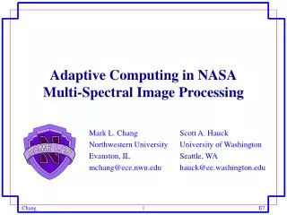
ACME LAB. Adaptive Computing in NASA Multi-Spectral Image Processing. Mark L. Chang Northwestern University Evanston, IL mchang@ece.nwu.edu. Scott A. Hauck University of Washington Seattle, WA hauck@ee.washington.edu. Background.

E N D
ACME LAB Adaptive Computing in NASAMulti-Spectral Image Processing Mark L. Chang Northwestern University Evanston, IL mchang@ece.nwu.edu Scott A. Hauck University of Washington Seattle, WA hauck@ee.washington.edu 1
Background • (1991) Initiative by NASA to study Earth as an environmental system—Earth Science Enterprise (ESE) • (1999) Launch of the first Earth Observation System (EOS) satellite, Terra 2
L2 L4 L1 L3 Receiver Level 0 Instrument 1 Instrument 2 Instrument 3 Instrument n The Data Flow • EOS divides telemetry processing into five levels with the following flow: 3
MODIS Instrument The Processing Problem • I/O intensive • Terra satellite generates ~918 Gbytes of data per day • Current NASA-supported data holdings total ~125,000 Gbytes • MODIS instrument accounts for over half the daily data and processing load 4
RAM RAM RAM RAM RAM RAM RAM RAM RAM RAM RAM RAM Why Adaptive Computing? • Instrument dependent processing • Data products involve many different algorithms • Algorithms often change over the lifetime of the instrument 5
MATCH Compiler • Current mappings are done by hand • Hardware description languages (Verilog, VHDL) • C program interface to adaptive compute engine • Requires low-level understanding of the architecture • MATCH == MATlab Compiler for Heterogeneous computing systems • MATLAB codes compiled to a configurable computing system automatically • Embedded processors, DSPs, and FPGAs • Performance goals • Within a factor of 2-4 of the best manual approach • Optimize performance under resource constraints 6
MATCH Compiler Framework • Parse MATLAB programs into intermediate representation • Build data and control dependence graph • Identify scopes for fine-grain, medium grain, and coarse grain parallelism • Map operations to multiple FPGAs, multiple embedded processors and multiple DSP processors • Automatic parallelization, scheduling, and mapping 7
MATCH Testbed Development Environment: SUN Solaris 2, HP HPUX and Windows Ultra C/C++ for MVME TI C for TMS320 XILINX XACT for XILINX • Annapolis Wildchild board • Nine XILINX 4010 FPGAs • 2 MB RAM • Wildfire software • Transtech TDMB 428 • DSP board • Four TDM 411 cards containing TI TMS 320C4 DSP, 8 MB RAM • TI C compiler • Motorola MVME-2604 • embedded boards • IBM PowerPC 604 • 64 MB RAM • OS-9 OS • Ultra C compiler Force 5V MicroSPARC CPU 64 MB RAM VME bus and chassis 8
Motivation for MATCH • NASA scientists prefer MATLAB • High-level language, good for prototyping and development • NASA applications are well-suited to the MATCH project • Lots of image and signal processing applications • Same domain as users of embedded systems • High degree of data parallelism • Small degree of task parallelism • NASA has an interest in adaptive technologies (ASDP) • Will be a benchmark for the MATCH compiler 9
Multi-spectral Image Classification • Want to classify a multi-spectral image in order to make it more useful for analysis by humans • Used to determine type of terrain being represented • Similar to data compression • Similar to clustering analysis Pixel[000][000] = ForestPixel[123][123] = UrbanPixel[255][212] = TundraPixel[410][230] = Water etc… 10
MATLAB Iterative for p=1:rows*cols % load pixel to process pixel = data( (p-1)*bands+1:p*bands ); class_total = zeros(classes,1); class_sum = zeros(classes,1); % class loop for c=1:classes class_total(c) = 0; class_sum(c) = 0; % weight loop for w=1:bands:pattern_size(c)*bands-bands weight = class(c,w:w+bands-1); class_sum(c) = exp( -(k2(c)*sum( (pixel-weight').^2 ))) + class_sum(c); end class_total(c) = class_sum(c) * k1(c); end results(p) = find( class_total == max( class_total ) )-1; end 12
MATLAB Vectorized % reshape data weights = reshape(class',bands,pattern_size(1),classes); for p=1:rows*cols % load pixel to process pixel = data( (p-1)*bands+1:p*bands); % reshape pixel pixels = reshape(pixel(:,ones(1,patterns)), bands,pattern_size(1),classes); % do calculation vec_res = k1(1).*sum(exp( -(k2(1).*sum((weights-pixels).^2)) )); vec_ans = find(vec_res==max(vec_res))-1; results(p) = vec_ans; end 13
Band K2 Mult Accumulator Pixel Unit Memory K2[K] Weight Memory Memory PNN Square Controller Unit Subtraction PE0 PE1 # of bands times PE2 PE3 PE4 Unit Class Compare exp / K1[K] Class K1[K] Mem Accumulator K1 Mult exp Mult exp LUT # weights/class times Unit Unit Unit Result Memory Initial FPGA Mapping 5% 67% 85% 82% 82% 14
Band K2 Mult Accumulator Pixel Unit Memory K2[K] Weight Memory Memory PNN Square Controller Unit Subtraction PE0 PE1 # of bands times PE2 PE3 PE4 Unit Class Compare exp / K1[K] Class K1[K] Mem Accumulator K1 Mult exp Mult exp LUT # weights/class times Unit Unit Unit Result Memory Improving the Mapping • Improve speed of PNN • Utilize all eight processing elements • Time-multiplex low-rate functions • Vary precision of multipliers/lookups 1:1 1:1 1:4 1:4 1:20 15
Optimized Mapping PE1 Subtract Square PE2 Subtract Square PE0 PE5 PE6 PE7 PE7 Pixel Reader K2 Multiplier Exponent Lookup Class Accumulator K1 Multiplier Class Comparison PE3 Subtract Square 5% 85% 61% 54% 97% PE4 Subtract Square 75% 16
Results Raw Image Data Processed Image Reference: HP C180 Workstation 17
Results (Cont’d) Reference:MATCH Testbed Force 5V MicroSPARC CPU 64 MB RAM 18
Conclusions • NASA is interested in adaptive computing • NASA has many candidate applications • High processing loads and I/O requirements • Applications are well-suited for acceleration using adaptive computing • Scientists will want to write in MATLAB rather than C+VHDL • Good benchmarks for the MATCH compiler • Will help identify functions and procedures necessary for real-world applications 20