From Id/pH to Dataflow Graphs Arvind Computer Science & Artificial Intelligence Lab

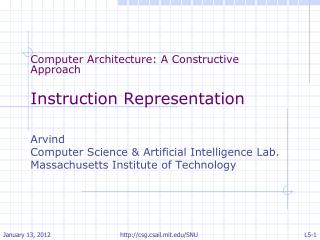
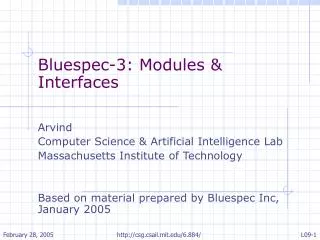
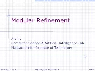
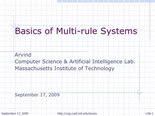
1. From Id/pH to Dataflow Graphs Arvind Computer Science & Artificial Intelligence Lab Massachusetts Institute of Technology http://csg.csail.mit.edu/arvind/

2. Tree of Activation Frames Global Heap of Shared Objects f: g: h: active threads asynchronous and parallel at all levels loop Parallel Language Model http://csg.csail.mit.edu/arvind/

3. Id Worldimplicit parallelism Id Dataflow Graphs + I-Structures + . . .TTDA Monsoon *T *T-Voyager http://csg.csail.mit.edu/arvind/

4. Id Compiler Phases Id desugar ß Kernel Id Reduction select representations ß Parallel Three Address Code, P-TAC ß Dataflow Graphs/Threads ß ß Fixed Program Machine Graphs von Neumann code Semantics of each intermediate language is important to show the correctness of each module http://csg.csail.mit.edu/arvind/

5. bounds 1. lower upper bounds lower upper 2. lower upper lower upper 3. 4. bounds array Choosing Representations: Arrays http://csg.csail.mit.edu/arvind/

6. Choosing Representations: Lists type list *0 = nil | cons *0 (list *0) Boxed 1. nil tag=0 Boxed cons tag=1 2. nil Unboxed tag Implicit cons Assumption: Pointers can be distinguished from small integers Similar issues arise for all Algebraic Types http://csg.csail.mit.edu/arvind/

7. Case Expression and Tags type foo .. = C1 ... | C2 ... | ... | Cn ... The case expression for type foo foo-case(d,e1,...,en) is implemented using the case construct: casek(i ,e1,...,ek) Þ ei where i = ifetch(d); http://csg.csail.mit.edu/arvind/

8. Top Level Functions f = lk(x1,...,xk).e Do not contain any free variables except the names of other top level functions. In general, its arguments can be supplied in one of two ways: 1. As a data structure which is built incrementally F = lxs.{ (x1,...,xk) = destruct(xs); in e } 2. All at once - fast call Ffc = lk(x1,...,xk).e http://csg.csail.mit.edu/arvind/

9. Multi-arity Functions def f x1 ... xk = e can be translated as f = lx1.lx2. ... lxk.e However, most implementation use k-arity ls f = lk(x1,...,xk).e with the rules: (lk(x1,...,xk).e) a Þ { x’1 = a in ((lk(x1,...,xk).e) x’1)} if k > 1 ((lk(x1,...,xk).e) x’1 ... x’n ) a Þ { x’n+1 = a in ((lk(x1,...,xk).e) x’1 ... x’n+1)} if n < k-1 ((lk(x1,...,xk).e) x’1 ... x’n ) a Þ { x’n+1 = a in e[x’1/x1]... [x’k/xk]} if n = k-1 Partial applications are values and thus substitutable http://csg.csail.mit.edu/arvind/

10. Loop Translation TE[{while epdo S finally ef } = { p = lk(x1,...,xk).TE[ep] ; b = lk(x1,...,xk). { TS[S] in nextx1,...,nextxk}; tp = p x ; t = Wloopk(p,b,x,tp) ; tf = TE[ef][t/x] ; in tf } where x = (x1,...,xk) and xi’s are the “nextified” variables of S and “next x” is replaced by “nextx” everywhere http://csg.csail.mit.edu/arvind/

11. Loop Rules Wloopk(p, b, x, true) Þ { t = b x; tp = p t; t’ = Wloopk(p, b, t, tp) in t’ } Wloopk(p, b, x, false) Þ x http://csg.csail.mit.edu/arvind/

12. KId - The Kernel Id LanguageAn extended lS-calculus E ::= x | lk(x1,...,xk).E | SE SE | { S in SE } | Casek(SE, E1,...,Ek) | PFk(SE1,...,SEk) | CN0 | CNk(SE1,...,SEk) | allocate() | Wloop(Ep,Eb,x,bool) S ::= x = E | S; S | S --- S | store(SE,SE,SE) PF2 ::= ...| i-fetch | m-fetch Simple Expressions SE ::= x | CN0 | CNk(SE1,...,SEk) | lk(x1,...,xk).E | ((lk(x1,...,xk).E) SE1...SEn) n < k http://csg.csail.mit.edu/arvind/

13. KId Optimizations “Totally correct” optimizations (lS rewrite rules) • Constant Propagation/Folding • Fetch Elimination • Barrier discharge • Inline Substitution/Specialization • Dead-code Elimination /Garbage collection ... Additional transformations or rewrite rules • Algebraic Identities • Common Subexpression Elimination • Code Hoisting out of Conditionals • Loop Optimizations • Peeling/Unrolling • Lifting loop invariants • Eliminating circulating variables and constants • Induction variable analysis http://csg.csail.mit.edu/arvind/

14. P-TAC: Three Address Code A lower level language than KId 1. Exposes all address calculations. Requires choosing representations for all data structures 2. No nested function definitions - l-abstractions exist only at the top level 3. Partial applications are represented as data structures (Closures) http://csg.csail.mit.edu/arvind/

15. . . . tg x1 xn G . . . sg Generating Dataflow Graphs GE :: P-TAC Expression --> DFG http://csg.csail.mit.edu/arvind/

16. c x1 x2 apply x1 ... xk PFk P-TAC to Dataflow GraphsExpressions x GE[c] = GE[x] = GE[x1 x2] = GE[PFk(x1,...,xk)] = http://csg.csail.mit.edu/arvind/

17. i x1 ... xn Switch 1 k x1 ... xn x1 ... xn ... GE[e1] GE[ek] Case Schema GE[Casek(i, e1,...,ek)] • { x1,...,xn } = FV(e1)U...U FV(ek) • All ei’s must have the same number of outputs • Unused xi’s in each branch have to be collected for signal generation http://csg.csail.mit.edu/arvind/

18. a a f f Þ apply get context extract tag x t: change Tag0 change Tag1 1: GE[e] 0: change Tag Graph for Function ApplicationThe Full Application case Apply is a conditional schema; make-closure part is not shown ((lk(x1,...,xk).e) x’1 ... x’k-1 ) a Þ { x’k = a in e[x’1/x1]... [x’k/xk] a new copy of e change tag http://csg.csail.mit.edu/arvind/ t

19. x1 ... xk tp next next next GS[Sb] GE[ep] Loop Schema GE[Wloopk(p,b,(x1,...,xk),tp] = ... • {x1,...,xn} are the nextified variables • p = lk(x1...xk).ep • b = lk(x1...xk).{Sb in next x1,...,next xk } ... http://csg.csail.mit.edu/arvind/

20. . . . tg x1 xn GS(S) . . . y1 ym x sg . . . tg x1 xn GE(e) x sg x1 x2 istore sg P-TAC to Dataflow GraphsThe Block Expression GE[{S in x}] = where {x1,...,xn} = FV(S) GS[x = e] = where {x1,...,xn} = FV(e) GS[store(x1,x2)] = http://csg.csail.mit.edu/arvind/

21. x1 ... xn . . . . . . tg x11 x1n tg x21 x2n GS(S1) GS(S2) . . . . . . y11 y1m sg y21 y2m sg Id y1 ... yn Parallel Composition ''Wiring Diagrams'' GS[S1;S2] = {y1,...,yn} = BV(S1) U BV(S2) {x1,...,xn} = FV(S1) U FV(S2) - {y1,...,yn} Each xij is to be connected to the yij with the same name http://csg.csail.mit.edu/arvind/

22. . . . tg x11 x1n GS(S1) . . . y11 y1m sg Sequential Composition GS[S1---S2] = x1 ... xn . . . tg x21 x2n GS(S2) . . . y21 y2m sg y1 ... yn {x1,...,xn} = FV(S1) U FV(S2) {y1,...,yn} = BV(S1) U BV(S2) Each x2j is to be connected to the y1j with the same name http://csg.csail.mit.edu/arvind/