Methods for the Study of Complex Systems

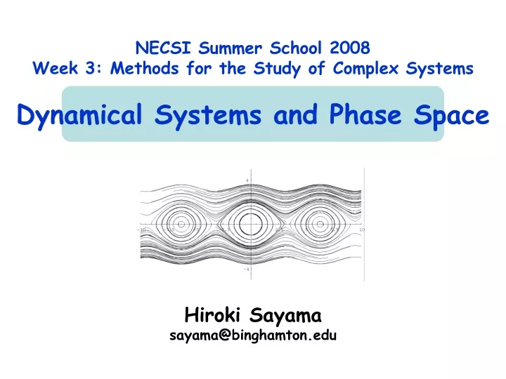
1. NECSI Summer School 2008Week 3: Methods for the Study of Complex SystemsDynamical Systems and Phase Space Hiroki Sayama sayama@binghamton.edu

2. Four approaches to complexity Nonlinear Dynamics Complexity = No closed-form solution, Chaos Information Complexity = Length of description, Entropy Computation Complexity = Computational time/space, Algorithmic complexity Collective Behavior Complexity = Multi-scale patterns, Emergence

3. Mathematical formulations of dynamical systems • Discrete-time model: xt = F(xt-1, t) • Continuous-time model: (differential equations) dx/dt = F(x, t) xt: State variable of the system at time t • May take “scalar” or “vector” value F: Some function that determines the rule that the system’s behavior will obey (difference/recurrence equations; iterative maps)

4. Geometrical Approach to Dynamical Systems

5. Geometrical approach • Developed in the late 19C by J. Henri Poincare • Visualizes the behavior of dynamical systems as trajectories in a phase space • Produces a lot of intuitive insights on geometrical structure of dynamics that would be hard to infer using purely algebraic methods

6. Phase space (state space) • A theoretical space in which every state of a dynamical system is mapped to a spatial location • Created by orthogonalizing state variables of the system; its dimensionality equals # of variables needed to specify the system state (a.k.a. degree of freedom) • Temporal change of the system states can be drawn in it as a trajectory

7. Attractor and basin of attraction • Attractor: A state (or a set of states) from which no outgoing edges or flows running in phase space • Static attractors (equilibrium points) • Dynamic attractors (e.g. limit cycles) • Basin of attraction: A set of states which will eventually end up in a given attractor

8. Visualizing Phase Space of Discrete Models

9. Phase space of discrete models • E.g. a simple blinking light • State can be specified by one binary variable (on or off) on off Dynamics of discrete-state models can be depicted as a directed graph (“state-transition diagram”) whose nodes/edges represent states/transitions (For stochastic systems one node may have multiple outgoing edges)

10. Exercise • Components A & B takes either red or blue Interaction rules are defined as follows: • A tries to be the same color as its partner • B tries to be the opposite color to its partner • Draw a phase space and trajectories of this system A B

11. Exercise • Think about: • How many independent variables? • How many possible system states? • What kind of phase space to be used? A B

12. A A A B B B A B Answer B A

13. Exercise: Three-person majority game • There is a group made of three persons • Each person takes either option X or Y • Each person makes his/her choices open to the other two, then they simultaneously switch their choices to the major option within the group • This process repeats indefinitely • Illustrate geometrical structure of the phase space of this system and identify attractors and basins of attractions in it

14. AAA AAB ABA BAA ABB BAB BBA BBB Answer

15. AAA AAB ABA BAA ABB BAB BBA BBB Answer Basin of attraction of Attractor A Attractor A Attractor B Basin of attraction of Attractor B

16. Exercise • Illustrate geometrical structure of the phase space of a three-person minoritygame (i.e., each person switches his/her choice against the major option within the group)

17. Answer Dynamic attractor BAA BAB AAA AAB BBA BBB ABA ABB There is only one basin of attraction in this case

18. Exercise • Four persons form a social contact network as shown on the left • When someone catches cold, she will get well after one time step, but cold will infect all of her healthy neighbors • Illustrate geometrical structure of the phase space of this system

19. Reducing the number of states • In some cases, it may be possibleto reduce the number of possible states by using symmetries • Rotational • Reflectional • Translational • Graph isomorphism etc.

20. Exercise • Reduce the number of possible states of the previous “cold network” example using symmetries

21. Visualizing Phase Space of Continuous Models

22. Phase space of continuous models • E.g. a simple vertical spring oscillator • State can be specified by two real variables (location x, velocity v) x Trajectory (orbit) v Dynamics of continuous models can be depicted as “flow” in a continuous phase space

23. Visualizing phase space of continuous models manually • Find “nullclines” • Points in the phase space where one of the derivatives is zero (i.e., trajectories are in parallel to one of the axes) • Plot where the nullclines are • Find how the sign of the derivative changes across the nullclines • Find values of other non-zero derivatives • Draw a “flow” between those nullclines with curves that don’t intersect with each other

24. Exercise • Draw an outline of the phase space of the following system by studying the distribution of its nullclines: dx/dt = x – x y dy/dt = y – x y (x >= 0, y >= 0)

25. Visualizing phase space of continuous models • Vector field • Uses many small arrows to show how local derivatives (or direction of trajectories) change from place to place in phase space • Phase portrait • Shows several typical trajectories to illustrate how phase space is globally structured

26. Exercise: Draw a phase space of the SIR model • “Susceptible” individuals can turn into “Infective” by contacting other “Infectives” • “Infective” individuals turn into “Removed” at a given rate • dS/dt = -i S I • dI/dt = i S I – r I • dR/dt = r I

27. Exercise: Draw a phase space of the RPS model • Assume a cyclic food chain among three species so that “Rock” eat “Scissors”, “Scissors” eat “Paper”, and “Paper” eat “Rock” • Each species will increase by eating other species and decrease by being eaten by others • dR/dt = a R S – b R P • dP/dt = b R P – c S P • dS/dt = - a R S + c S P

28. Summary: Advantage of geometrical approach • By using phase space, one can convert dynamic behaviors of systems into a static picture • By identifying geometrical structure of phase space such as attractors and basins of attraction, one can visually describe possible final states of the system and its sensitivity to initial conditions

29. Linear Systems

30. Linear systems • Linear systems are the simplest cases where states of nodes are continuous-valued and their dynamics are described by a time-invariant matrix • Discrete-time: xt = Axt-1 • Continuous-time: dx/dt = Bx • A / B are called “coefficient” matrices • We don’t consider constants (as they can be easily converted to the above forms)

31. s1 Example: An “averaging” network • A discrete-time dynamical network where the next state of each node is an average of its neighbors’ states (including its own) : s1 s2 s5 s1t = { s1t-1 + s2t-1 + s3t-1 + s5t-1 } / 4 s3 s4

32. s1 Exercise • Write down the state-transition function of the following “averaging” network by completing its coefficient matrix s1 s2 s5 s = {s1, s2, s3, s4, s5} st = (???) st-1 s3 s4

33. s1 Exercise • Derive the coefficient matrix of a similar “averaging” dynamical network that behaves in continuous time s1 s1 s1 s1 s2 s5 s = {s1, s2, s3, s4, s5} ds/dt = (???) s s3 s4

34. Coefficient matrix and adjacency matrix • Coefficient matrices are very similar to adjacency matrices of graphs: • If there is no interaction (= no edge) between nodes j and i, then aij = 0 • A weight aij in an adjacency matrix corresponds to the strength of influence from node j to i • One difference: A coefficient matrix may take negative components in it

35. Equilibrium points of linear systems • Discrete-time: xt = Axt-1 • Continuous-time: dx/dt = Bx • Linear systems have the origin (x=0) as a trivial equilibrium point • Can they have other non-trivial (non-zero) equilibrium points?

36. Finding equilibrium points • Discrete-time: xt = Axt-1 • Continuous-time: dx/dt = Bx • Discrete-time: xe = Axe • Continuous-time: 0 = B xe • If A has 1 (or if B has 0) as its eigenvalue, then the corresponding eigenvector(s) show the system’s equilibrium point(s)

37. Exercise • Obtain equilibrium points of the “averaging” network in both discrete- and continuous-time cases s1 s2 s5 s3 s4

38. Asymptotic Behavior of Linear Systems

39. Where will the system go eventually? • Discrete-time: xt = Axt-1 • Continuous-time: dx/dt = Bx These equations give the following exact solutions: • Discrete-time: xt = At x0 • Continuous-time: xt = eBt x0 = { I + Sk=1~(Bt)k/k! } x0

40. FYI: Exponential operator for matrices • xt =eBt x0 = { I + Sk=1~(Bt)k / k! } x0 • Similar to the Taylor series expansion of the exponential function: ex = 1+ x + x2/2! + x3/3! + … • eM converges for any square matrix M • If M’s eigenvalues are {li }, then eM’s eigenvalues are { eli}, with all eigenvectors unchanged (you can prove this)

41. Where will the system go eventually? • Discrete-time: xt = Axt-1 • Continuous-time: dx/dt = Bx • What happens if the system starts from non-equilibrium initial states and goes on for a long period of time? • Let’s think about their asymptotic behavior lim t->xt!!

42. Considering asymptotic behavior (1) • Let { vi } be nlinearly independent eigenvectors of the coefficient matrix (They might be fewer than n, but here we ignore such cases for simplicity) • Write the initial condition using eigenvectors, i.e. x0 = b1v1 + b2v2 + ... + bnvn

43. Considering asymptotic behavior (2) • Then: xt = At x0(discrete-time) =l1t b1v1 + l2t b2v2 + … + lnt bnvn or xt = eBt x0(continuous-time) = el1t b1v1 +el2t b2v2 + … +elnt bnvn

44. Dominant eigenvector (1) • Discrete-time: If |l1| > |l2|, |l3|, …, xt = l1t { b1v1 + (l2/l1)t b2v2 + ... + (ln/l1)t bnvn } lim t->xt ~ l1t b1v1 • Continuous-time: If Re(l1) > Re(l2), Re(l3), …, xt = el1t {b1v1 +e(l2-l1)t b2v2 + ... +e(ln-l1)t bnvn } lim t->xt ~ el1t b1v1 If the system has just one such dominant eigenvector v1, its state will be eventually along that vectorregardless of where it starts

45. Dominant eigenvector (2) • If the system has just one such dominant eigenvector v1, its state will be eventually along that vectorregardless of where it starts • But divergence or oscillation are possible • If, additionally, l1=1 (discrete-time) or 0 (continuous-time), then the system will eventually reach the equilibrium point (If the system has multiple dominant eigenvectors, final states may depend on initial states)

46. FYI: What eigenvalues and eigenvectors can tell us • An eigenvalue tells whether a particular “state” of the system (specified by its corresponding eigenvectors) grows or shrinks by interactions between parts • | l | > 1 -> growing • | l | < 1 -> shrinking • Re(l) > 0 -> growing • Re(l) < 0 -> shrinking for discrete-time cases for continuous-time cases

47. Along these lines (called invariant lines), the dynamics can be understood as simple exponential growth/decay |l1|>1 |l2|<1 v1 v2 Example • Phase space of a two-variable linear difference equation with (a, b, c, d) = (1, 0.1, 0.1, 0.9) y x

48. Example y x This could be regarded as a very simple form of self-organization (though completely predictable); Order spontaneously emerges in the system as time goes on

49. Exercise • Calculate eigenvalues of the following linear system and predict its dynamics along the lines given by the eigenvectors xt = 2 xt-1 - 2 yt-1 yt = 0.2 xt-1 + 0.2 yt-1 • Draw its phase space to confirm your prediction

50. Exercise • Obtain asymptotic behavior of the following dynamical network (figures denote symmetric coefficients in A/B) in both discrete- and continuous-time cases 1 -1 0 1 1 -3