Download
1 / 157
1.73k likes | 2.12k Views
OCEAN WAVE FORECASTING AT E.C.M.W.F. Jean-Raymond Bidlot Marine Aspects Section European Centre for Medium-range Weather Forecasts. Resources:. Lecture notes available at: http://www.ecmwf.int/newsevents/training/lecture_notes/ pdf_files /NUMERIC/Wave_mod.pdf

E N D
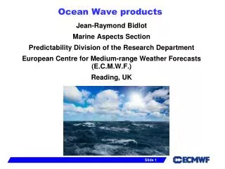
OCEAN WAVE FORECASTING AT E.C.M.W.F. Jean-Raymond Bidlot Marine Aspects Section European Centre for Medium-range Weather Forecasts
Resources: Lecture notes available at:http://www.ecmwf.int/newsevents/training/lecture_notes/pdf_files/NUMERIC/Wave_mod.pdf Model documentation available at:http://www.ecmwf.int/research/ifsdocs/CY38r1/index.html Ocean wave Forecasting at ECMWF
Directly Related Books: • “Dynamics and Modelling of Ocean Waves”. by: G.J. Komen, L. Cavaleri, M. Donelan, K. Hasselmann, S. Hasselmann, P.A.E.M. Janssen. Cambridge University Press, 1996. • “The Interaction of Ocean Waves and Wind”. By: Peter Janssen Cambridge University Press, 2004. Ocean wave Forecasting at ECMWF
earthquake Forcing: moon/sun wind Restoring: gravity surface tension Coriolis force 10.0 1.0 0.03 3x10⁻³ 2x10⁻⁵ 1x10⁻⁵ Frequency (Hz) What we are dealing with Ocean wave Forecasting at ECMWF
Water surfaceelevation, Wave Period, T Wave Length, Wave Height, H What we are dealing with Wave number: k = 2 π / λWave (angular) frequency: ω = 2 π / T Ocean wave Forecasting at ECMWF
What we are dealing with Ocean wave Forecasting at ECMWF
What we are dealing with Ocean wave Forecasting at ECMWF
What we are dealing with Ocean wave Forecasting at ECMWF
What we are dealing with Ocean wave Forecasting at ECMWF
Ocean waves: We are dealing with wind generated waves at the surface of the oceans, from gentle to rough … Ocean wave Forecasting at ECMWF
Individual waves Hmax Hs= H1/3 … etc. A Wave RecordIndividual Waves,Significant Wave Height, Hs,Maximum Individual Wave Height, Hmax Surface elevation time series from platform Draupner in the North Sea Ocean wave Forecasting at ECMWF
The distribution of wave energy among those components is called: “wave spectrum”, F(f,). Wave Spectrum • The irregular water surface can be decomposed into (infinite) number of simple sinusoidal components with different frequencies (f) and propagation directions ( ). Ocean wave Forecasting at ECMWF
Modern ocean wave prediction systems are based on statistical description of oceans waves (i.e. ensemble average of individual waves). • The sea state is described by the two-dimensional wave spectrum F(f,). Ocean wave Forecasting at ECMWF
What we are dealing with Ocean wave Forecasting at ECMWF
What we aredealing with Ocean wave Forecasting at ECMWF
What we are (not) dealing with (this week) Ocean wave Forecasting at ECMWF
Program of the lectures: 1. Derivation of energy balance equation 1.1. Preliminaries- Basic Equations- Dispersion relation in deep & shallow water.- Group velocity.- Energy density.- Hamiltonian & Lagrangian for potential flow.- Average Lagrangian.- Wave groups and their evolution. Ocean wave Forecasting at ECMWF
Program of the lectures: 1. Derivation of energy balance equation 1.2. Energy balance Eq. - Adiabatic Part - Need of a statistical description of waves: the wave spectrum.- Energy balance equation is obtained from averaged Lagrangian.- Advection and refraction. Ocean wave Forecasting at ECMWF
Program of the lectures: 1. Derivation of energy balance equation 1.3. Energy balance Eq. - Physics Diabatic rate of change of the spectrum determined by: - energy transfer from wind (Sin) - non-linear wave-wave interactions (Snonlin) - dissipation by white capping (Sdis). Ocean wave Forecasting at ECMWF
Program of the lectures: 1. Derivation of energy balance equation 1.4. Energy balance for wind sea - Wind sea and swell.- Empirical growth curves.- Energy balance for wind sea.- Evolution of wave spectrum.- Comparison with observations (JONSWAP). Ocean wave Forecasting at ECMWF
Program of the lectures: 2. Wave Forecasting at ECMWF 2.1 Operational configurations - Limited area model - Global, coupled to atmospheric model Ocean wave Forecasting at ECMWF
Program of the lectures: 2. Wave Forecasting at ECMWF 2.2 ECWAM - Wind input - Feedback to the atmosphere (two-way coupling) - Swell damping - Non linear source term - Bottom effects - Feedback on SST. Ocean wave Forecasting at ECMWF
Program of the lectures: 3. Validation 3.1. Use as a diagnostic tool 3.2. Comparison to observations - in-situ - Altimeter - Buoy spectra Ocean wave Forecasting at ECMWF
Program of the lectures: 4. Future developments 4.1. Impact on ocean circulation 4.2. Unstructured grid 4.3. wave – sea ice interaction Ocean wave Forecasting at ECMWF
1. Derivation of the Energy Balance Eqn: Solve problem with perturbation methods:(i) a / w << 1 (ii) s << 1 Lowest order: free gravity waves. Higher order effects: wind input, nonlinear transfer & dissipation Ocean wave Forecasting at ECMWF
Deterministic Evolution Equations • Result: Application to wave forecasting is a problem: 1. Do not know the phase of waves Spectrum F(k) ~ a*(k) a(k) Statistical description 2. Direct Fourier Analysis gives too many scales: Wavelength: 1 - 250 m Ocean basin: 107 m 2D 1014 equations Multiple scale approach · short-scale, O(), solved analytically · long-scale related to physics. Result: Energy balance equation that describes large-scale evolution of the wave spectrum. Ocean wave Forecasting at ECMWF
1.1. Preliminaries: • Interface between air and ocean: • Incompressible two-layer ideal fluid • Navier-Stokes:Here and surface elevation follows from: • Oscillations should vanish for:z± and z = -D (bottom) • No stresses; a 0 ; irrotational potential flow: (velocity potential )Then, obeys potential equation. Ocean wave Forecasting at ECMWF
Laplace’s Equation • Conditions at surface: • Conditions at the bottom: • Conservation of total energy:with the energy density z Ocean wave Forecasting at ECMWF
Hamilton Equations:Choose as variables: and Boundary conditions then follow from Hamilton’s equations:Advantage of this approach: Solve Laplace equation with boundary conditions: = (,). Then evolution in time follows from Hamilton equations. Ocean wave Forecasting at ECMWF
Lagrange FormulationVariational principle:with:gives Laplace’s equation & boundary conditions. Ocean wave Forecasting at ECMWF
V(q) • IntermezzoClassical mechanics: Particle (p,q) in potential well V(q)Total energy: Regard p and q as canonical variables. Hamilton’s equations are: Eliminate p Newton’s law = Force Ocean wave Forecasting at ECMWF
Principle of “least” action. Lagrangian:Newton’s law Action is extreme, whereAction is extreme if (action) = 0, where This is applicable for arbitrary q hence (Euler-Lagrange equation) Ocean wave Forecasting at ECMWF
Define momentum, p, as:and regard now p and q are independent, the Hamiltonian, H , is given as:Differentiate H with respect to q givesThe other Hamilton equation:All this is less straightforward to do for a continuum. Nevertheless, Miles obtained the Hamilton equations from the variational principle.Homework: Derive the governing equations for surface gravity waves from the variational principle. Ocean wave Forecasting at ECMWF
Linear TheoryLinearized equations become:Elementary sineswhere a is the wave amplitude, is the wave phase.Laplace: Ocean wave Forecasting at ECMWF
Constant depth: z= -DZ'(-D) = 0 Z ~ cosh [ k (z+D)] with and Dispersion Relation finally Deep waterShallow water D D0 • dispersion relation: • phase speed: group speed: Note: • low freq. waves faster ! No dispersion. • energy: Ocean wave Forecasting at ECMWF
(t) t Slight generalisation: Slowly varying depth and/or current, , = intrinsic frequency • Wave GroupsSo far a single wave. However, waves come in groups.Long-wave groups may be described with geometrical optics approach:Amplitude and phase vary slowly: Ocean wave Forecasting at ECMWF
Local wave number and phase (recall wave phase !) Consistency: conservation of number of wave crests Slow time evolution of amplitude is obtained by averaging the Lagrangian over rapid phase, . For water waves we get (after dropping the brackets )with Ocean wave Forecasting at ECMWF
In other words, we have(omitting the brackets ) Evolution equations then follow from the average variational principle We obtain:a : (dispersion relation) : (evolution of amplitude) plus consistency: (conservation of crests) Finally, if we introduce a transport velocity thenL is called the action density. Ocean wave Forecasting at ECMWF
Apply our findings to gravity waves. Linear theory, write L aswhere Dispersion relation follows fromhence, with , Equation for action density, N,becomeswith Closed by Ocean wave Forecasting at ECMWF
Consequencies Zero flux through boundaries hence, in case of slowly varying bottom and currents, the wave energy is not constant. Of course, the total energy of the system, including currents, ... etc., is constant. However, when waves are considered in isolation (regarded as “the” system), energy is not conserved because of interaction with current (and bottom). The total action density is Ntot is conserved. The action density is called an adiabatic invariant. Ocean wave Forecasting at ECMWF
Homework: Adiabatic Invariants(study this) Consider once more the particle in potential well. Externally imposed change (t). We have Variational equation is Calculate average Lagrangian with fixed. If period is = 2/ , then For periodic motion ( = const.) we have conservation of energythus also momentum is The average Lagrangian becomes Ocean wave Forecasting at ECMWF
Allow now slow variations of which give consequent changes in E and . Average variational principle Define again Variation with respect to E & gives The first corresponds to the dispersion relation while the second corresponds to the action density equation. Thus which is just the classical result of an adiabatic invariant. As the system is modulated, and E vary individually but remains constant: Analogy LL waves. Example: Pendulum with varying length! Ocean wave Forecasting at ECMWF
(t) t Wave packet evolution: Local wave number and phase: Consistency: Dispersion relation: Equation for action density: Ocean wave Forecasting at ECMWF
1.2. Energy Balance Eqn (Adiabatic Part): • Together with other perturbations where wave number and frequency of wave packet follow from So far we were solving for • Statistical description of waves: concept of the wave spectrum • Random phase Gaussian surface • Covariance homogeneouswith = ensemble average depends only on Ocean wave Forecasting at ECMWF
• By definition, wave number spectrum is the Fourier transform of correlation RWe now take a continuum of waves. Realising that we have two modes : is real Use this in homogeneous two point correlation, we must have and the correlation becomes Ocean wave Forecasting at ECMWF