Download
1 / 21
210 likes | 494 Views
Disks. Overview of Mass-Storage Structure In this section we present a general overview of the physical structure of secondary and tertiary storage devices. Magnetic Disks

E N D
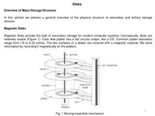
Disks Overview of Mass-Storage Structure In this section we present a general overview of the physical structure of secondary and tertiary storage devices. Magnetic Disks Magnetic disks provide the bulk of secondary storage for modern computer systems. Conceptually, disks are relatively simple (Figure 1). Each disk platter has a flat circular shape, like a CD. Common platter diameters range from 1.8 to 5.25 inches. The two surfaces of a platter are covered with a magnetic material. We store information by recording it magnetically on the platters. Fig. 1 Moving-head disk mechanism
A read write head "flies" just above each surface of every platter. The heads are attached to a disk arm that moves all the heads as a unit. The surface of a platter is logically divided into circular tracks, which are subdivided into sectors. The set of tracks that are at one arm position makes up a cylinder. There may be thousands of concentric cylinders in a disk drive, and each track may contain hundreds of sectors. The storage capacity of common disk drives is measured in gigabytes. When the disk is in use, a drive motor spins it at high speed. Most drives rotate 60 to 200 times per second. Disk speed has two parts. The transfer rate is the rate at which data flow between the drive and the computer. The positioning time, sometimes called the random-access time, consists of the time to move the disk arm to the desired cylinder, called the seek time, and the time for the desired sector to rotate to the disk head, called the rotational latency. Typical disks can transfer several megabytes of data per second, and they have seek times and rotational latencies of several milliseconds. Because the disk head flies on an extremely thin cushion of air (measured in microns), there is a danger that the head will make contact with the disk surface. Although the disk platters are coated with a thin protective layer, sometimes the head will damage the magnetic surface. This accident is called a head crash. A head crash normally cannot be repaired; the entire disk must be replaced. A disk can be removable, allowing different disks to be mounted as needed. Removable magnetic disks generally consist of one platter, held in a plastic case to prevent damage while not in the disk drive. Floppy disks are inexpensive removable magnetic disks that have a soft plastic case containing a flexible platter. The head of a floppy-disk drive generally sits directly on the disk surface, so the drive is designed to rotate more slowly than a hard-disk drive to reduce the wear on the disk surface. The storage capacity of a floppy disk is typically only 1.44 MB or so. Removable disks are available that work much like normal hard disks and have capacities measured in gigabytes. A disk drive is attached to a computer by a set of wires called an I/O bus. Several kinds of buses are available, including enhanced integrated drive electronics (EIDE), advanced technology attachment (ATA), serial ATA (SATA), universal serial bus (USB), fiber channel (FC), and SCSI buses. The data transfers on a bus are carried out by special electronic processors called controllers. The host controller is the controller at the computer end of the bus. A disk controller is built into each disk drive. To perform a disk I/O operation, the computer places a command into the host controller, typically using memory-mapped I/O ports. The host controller then sends the command via messages to the disk controller, and the disk controller operates the disk-drive hardware to carry out the command.
Magnetic Tapes Magnetic tape was used as an early secondary-storage medium. Although it is relatively permanent and can hold large quantities of data, its access time is slow compared with that of main memory and magnetic disk. In addition, random access to magnetic tape is about a thousand times slower than random access to magnetic disk, so tapes are not very useful for secondary storage. Tapes are used mainly for backup, for storage of infrequently used information, and as a medium for transferring information from one system to another. A tape is kept in a spool and is wound or rewound past a read-write head. Moving to the correct spot on a tape can take minutes, but once positioned, tape drives can write data at speeds comparable to disk drives. Tape capacities vary greatly, depending on the particular kind of tape drive. Typically, they store from 20 GB to 200 GB. Some have built-in compression that can more than double the effective storage. Tapes and their drivers are usually categorized by width, including 4, 8, and 19 millimeters and 1/4 and 1/2 inch. Some are named according to technology, such as LTO-2 and SDLT. Disk Structure Modern disk drives are addressed as large one-dimensional arrays of logical blocks, where the logical block is the smallest unit of transfer. The size of a logical block is usually 512 bytes, although some disks can be low-level formatted to have a different logical block size, such as 1,024 bytes. The one-dimensional array of logical blocks is mapped onto the sectors of the disk sequentially. Sector 0 is the first sector of the first track on the outermost cylinder. The mapping proceeds in order through that track, then through the rest of the tracks in that cylinder, and then through the rest of the cylinders from outermost to innermost. By using this mapping, we can - at least in theory - convert a logical block number into an old-style disk address that consists of a cylinder number, a track number within that cylinder, and a sector number within that track. In practice, it is difficult to perform this translation, for two reasons. First, most disks have some defective sectors, but the mapping hides this by substituting spare sectors from elsewhere on the disk. Second, the number of sectors per track is not a constant on some drives.
Let's look more closely at the second reason. On media that use constant linear velocity (CLV), the density of bits per track is uniform. The farther a track is from the center of the disk, the greater its length, so the more sectors it can hold. As we move from outer zones to inner zones, the number of sectors per track decreases. Tracks in the outermost zone typically hold 40 percent more sectors than do tracks in. the innermost zone. The drive increases its rotation speed as the head moves from the outer to the inner tracks to keep the same rate of data moving under the head. This method is used in CD-ROM and DVD-ROM drives. Alternatively, the disk rotation speed can stay constant, and the density of bits decreases from inner tracks to outer tracks to keep the data rate constant. This method is used in hard disks and is known as constant angular velocity (CAV). Computers access disk storage in two ways. One way is via I/O ports (or host-attached storage); this is common on small systems. The other way is via a remote host in a distributed file system; this is referred to as network-attached storage. Host-Attached Storage Host-attached storage is storage accessed through local I/O ports. These ports use several technologies. The typical desktop PC uses an I/O bus architecture called IDE or ATA. This architecture supports a maximum of two drives per I/O bus. A newer, similar protocol that has simplified cabling is SATA. High-end workstations and servers generally use more sophisticated I/O architectures, such as SCSI and fiber channel (FC). SCSI is a bus architecture. Its physical medium is usually a ribbon cable having a large number of conductors (typically 50 or 68). The SCSI protocol supports a maximum of 16 devices on the bus. Generally, the devices include one controller card in the host (the SCSI initiator) and up to 15 storage devices (the SCSI targets). A SCSI disk is a common SCSI target, but the protocol provides the ability to address up to 8 logical units in each SCSI target. A typical use of logical unit addressing is to direct commands to components of a RAID array or components of a removable media library (such as a CD jukebox sending commands to the media-changer mechanism or to one of the drives). FC is a high-speed serial architecture that can operate over optical fiber or over a four-conductor copper cable. It has two variants. One is a large switched fabric having a 24-bit address space. This variant is expected to dominate in the future and is the basis of storage-area networks (SANs). Because of the large address space and the switched nature of the communication, multiple hosts and storage devices can attach to the fabric, allowing great flexibility in I/O communication. The other PC variant is an arbitrated loop (FC-AL) that can address 126 devices (drives and controllers).
A wide variety of storage devices are suitable for use as host-attached storage. Among these are hard disk drives, RAID arrays, and CD, DVD, and tape drives. The I/O commands that initiate data transfers to a host-attached storage device are reads and writes of logical data blocks directed to specifically identified storage units (such as bus ID, SCSI ID, and target logical unit). Network-Attached Storage A network-attached storage (NAS) device is a special-purpose storage system, that is accessed remotely over a data network (Figure 2). Clients access network-attached storage via a remote-procedure-call interface such as NFS for UNIX systems or CIFS for Windows machines. The remote procedure calls (RPCs) are carried via TCP or UDP over an IP network - usually the same local - area network (LAN) that carries all data traffic to the clients. The network-attached storage unit is usually implemented as a RAID array with software that implements the RPC interface. It is easiest to think of NAS as simply another storage-access protocol. For example, rather than using a SCSI device driver and SCSI protocols to access storage, a system using NAS would use RPC over TCP/IP. Figure 2. Network-attached storage Network-attached storage provides a convenient way for all the computers on a LAN to share a pool of storage with the same ease of naming and access enjoyed with local host-attached storage. However, it tends to be less efficient and have lower performance than some direct-attached storage options.
ISCSI is the latest network-attached storage protocol. In essence, it uses the IP network protocol to carry the SCSI protocol. Thus, networks rather than SCSI cables can be used as the interconnects between hosts and their storage. As a result, hosts can treat their storage as if it were directly attached, but the storage can be distant from the host. Storage-Area Network One drawback of network-attached storage systems is that the storage I/O operations consume bandwidth on the data network, thereby increasing the latency of network communication. This problem can be particularly acute in large client - server installations - the communication between servers and clients competes for bandwidth with the communication among servers and storage devices. A storage-area network (SAN) is a private network (using storage protocols rather than networking protocols) connecting servers and storage units, as shown in Figure 3. The power of a SAN lies in its flexibility. Multiple hosts and multiple storage arrays can attach to the same SAN, and storage can be dynamically allocated to hosts. A SAN switch allows or prohibits access between the hosts and the storage. As one example, if a host is running low on disk space, the SAN can be configured to allocate more storage to that host. SANs make it possible for clusters of servers to share the same storage and for storage arrays to include multiple direct host connections. SANs typically have more ports, and less expensive ports, than storage arrays. FC is the most common SAN interconnect. Figure 3. Storage-area Network
Disk Scheduling One of the responsibilities of the operating system is to use the hardware efficiently. For the disk drives, meeting this responsibility entails having fast access time and large disk bandwidth. The access time has two major components. The seek time is the time for the disk arm to move the heads to the cylinder containing the desired sector. The rotational latency is the additional time for the disk to rotate the desired sector to the disk head. The disk bandwidth is the total number of bytes transferred, divided by the total time between the first request for service and the completion of the last transfer. We can improve both the access time and the bandwidth by scheduling the servicing of disk I/O requests in a good order. Whenever a process needs I/O to or from the disk, it issues a system call to the operating system. The request specifies several pieces of information: • Whether this operation is input or output • What the disk address for the transfer is • What the memory address for the transfer is • What the number of sectors to be transferred is If the desired disk drive and controller are available, the request can be serviced immediately. If the drive or controller is busy, any new requests for service will be placed in the queue of pending requests for that drive. For a multiprogramming system with many processes, the disk queue may often have several pending requests. Thus, when one request is completed, the operating system chooses which pending request to service next. How does the operating system make this choice? Any one of several disk-scheduling algorithms can be used, and we discuss them next. FCFS Scheduling The simplest form, of disk scheduling is, of course, the first-come, first-served (FCFS) algorithm. This algorithm is intrinsically fair, but it generally does not provide the fastest service. Consider, for example, a disk queue with requests for I/O to blocks on cylinders 98, 183, 37, 122, 14, 124, 65, 67, in that order. If the disk head is initially at cylinder 53, it will first move from 53 to 98, then to 183, 37, 122, 14, 124, 65, and finally to 67, for a total head movement of 640 cylinders. This schedule is diagrammed in Figure 4.
Figure 4. FCSF disk scheduling The wild swing from 122 to 14 and then back to 124 illustrates the problem with this schedule. If the requests for cylinders 37 and 14 could be serviced together, before or after the requests at 122 and 124, the total head movement could be decreased substantially, and performance could be thereby improved. SSTF Scheduling It seems reasonable to service all the requests close to the current head position before moving the head far away to service other requests. This assumption is the basis for the shortest-seek-time-first (SSTF) algorithm. The SSTF algorithm selects the request with the minimum seek time from the current head position. Since seek time increases with the number of cylinders traversed by the head, SSTF chooses the pending request closest to the current head position. For our example request queue, the closest request to the initial head position (53) is at cylinder 65. Once we are at cylinder 65, the next closest request is at cylinder 67. From there, the request at cylinder 37 is closer than the one at 98, so 37 is served next. Continuing, we service the request at cylinder 14, then 98, 122, 124, and finally 183 (Figure 5). This scheduling method results in a total head movement of only 236 cylinders - little more than one-third of the distance needed for FCFS scheduling of this request queue. This algorithm gives a substantial improvement in performance.
SSTF scheduling is essentially a form of shortest-job-first (SJF) scheduling; and like SJF scheduling, it may cause starvation of some requests. Remember that requests may arrive at any time. Suppose that we have two requests in the queue, for cylinders 14 and 186, and while servicing the request from 14, a new request near 14 arrives. This new request will be serviced next, making the request at 186 wait. While this request is being serviced, another request close to 14 could arrive. In theory, a continual stream of requests near one another could arrive, causing the request for cylinder 186 to wait indefinitely. Figure 5. SSTF disk scheduling SCAN Scheduling In the SCAN algorithm, the disk arm starts at one end of the disk and moves toward the other end, servicing requests as it reaches each cylinder, until it gets to the other end of the disk. At the other end, the direction of head movement is reversed, and servicing continues. The head continuously scans back and forth across the disk. The SCAN algorithm is sometimes called the elevator algorithm, since the disk arm behaves just like an elevator in a building, first servicing all the requests going up and then reversing to service requests the other way.
Let's return to our example to illustrate. Before applying SCAN to schedule the requests on cylinders 98, 183, 37, 122, 14, 124, 65, and 67, we need to know the direction of head movement in addition to the head's current position (53). If the disk arm is moving toward 0, the head will service 37 and then 14. At cylinder 0, the arm will reverse and will move toward the other end of the disk, servicing the requests at 65, 67, 98, 122, 124, and 183 (Figure 6). If a request arrives in the queue just in front of the head, it will be serviced almost immediately; a request arriving just behind the head will have to wait until the arm moves to the end of the disk, reverses direction, and comes back. Assuming a uniform distribution of requests for cylinders, consider the density of requests when the head reaches one end and reverses direction. At this point, relatively few requests are immediately in front of the head, since these cylinders have recently been serviced. The heaviest density of requests is at the other end of the disk. These requests have also waited the longest, so why not go there first? That is the idea of the next algorithm. Figure 6. SCAN disk scheduling
C-SCAN Scheduling Circular SCAN (C-SCAN) scheduling is a variant of SCAN designed to provide a more uniform wait time. Like SCAN, C-SCAN moves the head from, one end of the disk to the other, servicing requests along the way. When the head reaches the other end, however, it immediately returns to the beginning of the disk, without servicing any requests on the return trip (Figure 7). The C-SCAN scheduling algorithm essentially treats the cylinders as a circular list that wraps around from the final cylinder to the first one. Figure 7. C-SCAN disk scheduling LOOK Scheduling As we described them, both SCAN and C-SCAN move the disk arm across the full width of the disk. In practice, neither algorithm is often implemented this way. More commonly, the arm goes only as far as the final request in each direction. Then, it reverses direction immediately, without going all the way to the end of the disk. Versions of SCAN and C-SCAN that follow this pattern are called LOOK and C-LOOK scheduling, because they look for a request before continuing to move in a given direction (Figure 8.)
Figure 8. LOOK disk scheduling Selection of a Disk-Scheduling Algorithm Given so many disk-scheduling algorithms, how do we choose the best one? SSTF is common and has a natural appeal because it increases performance over FCFS. SCAN and C-SCAN perform better for systems that place a heavy load on the disk, because they are less likely to cause a starvation problem. For any particular list of requests, we can define an optimal order of retrieval, but the computation needed to find an optimal schedule may not justify the savings over SSTF or SCAN. With any scheduling algorithm, however, performance depends heavily on the number and types of requests. For instance, suppose that the queue usually has just one outstanding request. Then, all scheduling algorithms behave the same, because they have only one choice for where to move the disk head: They all behave like FCFS scheduling. Because of these complexities, the disk-scheduling algorithm should be written as a separate module of the operating system, so that it can be replaced with a different algorithm if necessary. Either SSTF or LOOK is a reasonable choice for the default algorithm.
Disk Management The operating system is responsible for several other aspects of disk management, too. Here we discuss disk initialization, booting from disk, and bad-block recovery. Disk Formatting A new magnetic disk is a blank slate: It is just a platter of a magnetic recording material. Before a disk can store data, it must be divided into sectors that the disk controller can read and write. This process is called low-level formatting, or physical formatting. Low-level formatting fills the disk with a special data structure for each sector. The data structure for a sector typically consists of a header, a data area (usually 512 bytes in size), and a trailer. The header and trailer contain information used by the disk controller, such as a sector number and an error-correcting code (ECC). When the controller writes a sector of data during normal I/O, the ECC is updated with a value calculated from all the bytes in the data area. When the sector is read, the ECC is recalculated and is compared with the stored value. If the stored and calculated numbers are different, this mismatch indicates that the data area of the sector has become corrupted and that the disk sector may be bad. The ECC is an error-correcting code because it contains enough information that, if only a few bits of data have been corrupted, the controller can identify which bits, have changed and can calculate what their correct values should be. It then reports a recoverable soft error. The controller automatically does the ECC processing whenever a sector is read or written. Most hard disks are low-level-formatted at the factory as a part of the manufacturing process. This formatting enables the manufacturer to test the disk and to initialize the mapping front logical block numbers to defect-free sectors on the disk. For many hard disks, when the disk controller is instructed to low-level-format the disk, it can also be told how many bytes of data space to leave between the header and trailer of all sectors. It is usually possible to choose among a few sizes, such as 256, 512, and 1,024 bytes. Formatting a disk with a larger sector size means that fewer sectors can fit on each track; but it also means that fewer headers and trailers are written on each track and more space is available for user data. Some operating systems can handle only a sector size of 512 bytes.
Boot Block For a computer to start running - for instance, when it is powered up or rebooted - it must have an initial program to run. This initial bootstrap program tends to be simple. It initializes all aspects of the system, from CPU registers to device controllers arid the contents of main memory, and then starts the operating system. To do its job, the bootstrap program finds the operating-system kernel on disk, loads that kernel into memory, and jumps to an initial address to begin the operating-system execution. For most computers, the bootstrap is stored in read-only memory (ROM). This location is convenient, because ROM needs no initialization and is at a fixed location that the processor can start executing when powered up or reset. And, since ROM is read only, it cannot be infected by a computer virus. The problem is that changing this bootstrap code inquires changing the ROM hardware chips. For this reason, most systems store a tiny bootstrap loader program in the boot ROM whose only job is to bring in a full bootstrap program from disk. The full bootstrap program can be changed easily: A new version is simply written onto the disk. The full bootstrap program is stored in "the boot blocks" at a fixed location on the disk. A disk that has a boot partition is called a boot disk or system disk. The code in the boot ROM instructs the disk controller to read the boot blocks into memory (no device drivers are loaded at this point) and then starts executing that code. The full bootstrap program is more sophisticated than the bootstrap loader in the boot ROM; it is able to load the entire operating system from a non-fixed location on disk and to start the operating system running. Even so, the full bootstrap code may be small. Let's consider as an example the boot process in Windows. The Windows system places its boot code in the first sector on the hard disk (which it terms the master boot record, or MBR). Furthermore, Windows allows a hard disk to be divided into one or more partitions; one partition, identified as the boot partition, contains the operating system and device drivers. Booting begins in a Windows system by running code that is resident in the system's ROM memory. This code directs the system to read the boot code from the MBR. In addition to containing boot code, the MBR contains a table listing the partitions for the hard disk and a flag indicating which partition the system is to be booted from. This is illustrated in Figure 9. Once the system identifies the boot partition, it reads the first sector from that partition (which is called the boot sector) and continues with the remainder of the boot process, which includes loading the various subsystems and system services.
Figure 9. Booting from disk in Windows Bad Blocks Because disks have moving parts and small tolerances (recall that the disk head flies just above the disk surface), they are prone to failure. Sometimes the failure is complete; in this case, the disk needs to be replaced arid its contents restored from backup media to the new disk. More frequently, one or more sectors become defective. Most disks even come from the factory with bad blocks. Depending on the disk and controller in use, these blocks are handled in a variety of ways. On simple disks, such as some disks with IDE controllers, bad blocks are handled manually. For instance, the MS-DOS format command performs logical formatting and, as a part of the process, scans the disk to find bad blocks. If format finds a bad block, it writes a special value into the corresponding FAT entry to tell the allocation routines not to use that block. If blocks go bad during normal operation, a special program (such as ch.kd.sk) must be run manually to search for the bad blocks and to lock them away as before. Data that resided on the bad blocks usually are lost. More sophisticated disks, such as the SCSI disks used in high-end PCs and most workstations and servers, are smarter about bad-block recovery. The controller maintains a list of bad blocks on the disk. The list is initialized during the low-level formatting at the factory and is updated over the life of the disk. Low-level formatting also sets aside spare sectors not visible to the operating system. The controller can be told to replace each bad sector logically with one of the spare sectors. This scheme is known as sector sparing or forwarding.
A typical bad-sector transaction might be as follows: • The operating system tries to read logical block 87. • The controller calculates the ECC and finds that the sector is bad. It reports this finding to the operating system. • The next time the system is rebooted, a special command is run to tell the SCSI controller to replace the bad sector with, a spare. • After that, whenever the system requests logical block 87, the request is translated into the replacement sector's address by the controller. • Such a redirection by the controller could invalidate any optimization by the operating system's disk-scheduling algorithm! For this reason, most disks are formatted to provide a few spare sectors in each cylinder and a spare cylinder as well. When a bad block is remapped, the controller uses a spare sector from the same cylinder, if possible. • As an alternative to sector sparing, some controllers can be instructed to replace a bad block by sector slipping. Here is an example: Suppose that logical block 17 becomes defective and the first available spare follows sector 202. Then, sector slipping remaps all the sectors from 17 to 202, moving them all down one spot. That is, sector 202 is copied into the spare, then sector 201 into 202, and then 200 into 201, and so on, until sector 18 is copied into sector 19. Slipping the sectors in this way frees up the space of sector 18, so sector 17 can be mapped to it. • The replacement of a bad block generally is not totally automatic because the data in the bad block are usually lost. Several soft errors could trigger a process in which a copy of the block data is made and the block is spared or slipped. An unrecoverable hard error, however, results in lost data. Whatever file was using that block must be repaired (for instance, by restoration from a backup tape), and that requires manual intervention.
RAID Structure Disk drives have continued to get smaller and cheaper, so it is now economically feasible to attach many disks to a computer system. Having a large number of disks in a system presents opportunities for improving the rate at which data can be read or written, if the disks are operated in parallel. Furthermore, this setup offers the potential for improving the reliability of data storage, because redundant information can be stored on multiple disks. Thus, failure of one disk does not lead to loss of data. A variety of disk-organization techniques, collectively called redundant arrays of inexpensive disks (RAlDs), are commonly used to address the performance and reliability issues. In the past, RAIDS composed of small, cheap disks were viewed as a cost-effective alternative to large, expensive disks; today, RAIDs are used for their higher reliability and higher data-transfer rate, rather than for economic reasons. Hence, the I in RAID now stands for "independent" instead of "'inexpensive.'" Improvement of Reliability via Redundancy Let us first consider the reliability of RAlDs. The chance that some disk out of a set of TV disks will fail is much higher than the chance that a specific single disk will fail. Suppose that the mean time to failure of a single disk is 100,000 hours. Then the mean time to failure of some disk in an array of 100 disks will be 100,000/100 = 1,000 hours, or 41.66 days, which is not long at all! If we store only one copy of the data, then each disk failure will result in loss of a significant amount of data - and such a high rate of data loss is unacceptable. The solution to the problem of reliability is to introduce redundancy; we store extra information that is not normally needed but that can be used in the event of failure of a disk to rebuild the lost information. Thus, even if a disk fails, data are not lost. The simplest (but most expensive) approach to introducing redundancy is to duplicate every disk. This technique is called mirroring. A logical disk then consists of two physical disks, and every write is carried out on both disks. If one of the disks fails, the data can be read from the other. Data will be lost only if the second disk fails before the first failed disk is replaced. The mean time to failure - where failure is the loss of data - of a mirrored volume (made up of two disks, mirrored) depends on two factors. One is the mean time to failure of the individual disks. The other is the mean time to repair, which is the time it takes (on average) to replace a failed disk and to restore the data on it.
Suppose that the failures of the two disks are independent; that is, the failure of one disk is not connected to the failure of the other. Then, if the mean time to failure of a single disk is 100,000 hours and the mean time to repair is 10 hours, the mean time to data loss of a mirrored disk system is 100. 0002/(2 * 10) = 500 * 106 hours, or 57,000 years! You should be aware that the assumption of independence of disk failures is not valid. Power failures and natural disasters, such as earthquakes, fires, and floods, may result in damage to both disks at the same time. Also, manufacturing defects in a batch of disks can cause correlated failures. As disks age, the probability of failure grows, increasing the chance that a second disk will fail while the first is being repaired. In spite of all these considerations, however, mirrored-disk systems offer much higher reliability than do single-disk systems. Improvement in Performance via Parallelism Now let's consider how parallel access to multiple disks improves performance. With disk mirroring, the rate at which read requests can be handled is doubled, since read requests can be sent to either disk (as long as both disks in a pair are functional, as is almost always the case). The transfer rate of each read is the same as in a single-disk system, but the number of reads per unit time has doubled. With multiple disks, we can improve the transfer rate as well (or instead) by striping data across the disks. In its simplest form, data striping consists of splitting the bits of each byte across multiple disks; such striping is called bit-level striping. For example, if we have an array of eight disks, we write bit i of each byte to disk i. The array of eight disks can be treated as a single disk with sectors that are eight times the normal size and, more important, that have eight times the access rate. In such an organization, every disk participates in every access (read or write); so the number of accesses that can be processed per second is about the same as on a single disk, but each access can read eight times as many data in the same time as on a single disk. Bit-level striping can be generalized to include a number of disks that either is a multiple of 8 or divides 8. For example, if we use an array of four disks, bits i and 4 + i of each byte go to disk i. Further, striping need not be at the bit level. For example, in block-level striping, blocks of a file are striped across multiple disks; with n disks, block i of a file goes to disk (i mod n) + 1. Other levels of striping, such as bytes of a sector or sectors of a block, also are possible. Block-level striping is the most common. Parallelism in a disk system, as achieved through striping, has two main goals: 1. Increase the throughput of multiple small accesses (that is, page accesses) by load balancing. 2. Reduce the response time of large accesses.
RAID Levels Mirroring provides high reliability, but it is expensive. Striping provides high data-transfer rates, but it does not improve reliability. Numerous schemes to provide redundancy at lower cost by using the idea of disk striping combined with "parity" bits (which we describe next) have been proposed. These schemes have different cost - performance trade-offs and are classified according to levels called RAID levels. We describe the various levels here; Figure 10 shows them pictorially (in the figure, P indicates error-correcting bits, and C indicates a second copy of the data). In all cases depicted in the figure, four disks' worth of data are stored, and the extra disks are used to store redundant information for failure recovery. Figure 10. RAID levels
RAID Level 0. RAID level 0 refers to disk arrays with striping at the level of blocks but without any redundancy (such as mirroring or parity bits), as shown in Figure 10(a). • RAID Level 1. RAID level 1 refers to disk mirroring. Figure 10(b) shows a mirrored organization. • RAID Level 2. RAID level 2 is also known as memory-style error-correcting-code (ECC) organization. Memory systems have long detected certain errors by using parity bits. Each byte in a memory system may have a parity bit associated with it that records whether the number of bits in the byte set to 1 is even (parity = 0) or odd (parity = 1). If one of the bits in the byte is damaged (either a 1 becomes a 0, or a 0 becomes a 1), the parity of the byte changes and thus will not match the stored parity. Similarly, if the stored parity bit is damaged, it will not match the computed parity. Thus, all single-bit errors are detected by the memory system. Error-correcting schemes store two or more extra bits and can reconstruct the data if a single bit is damaged. The idea of ECC can be used directly in disk arrays via striping of bytes across disks. For example, the first bit of each byte can be stored in disk 1, the second bit in disk 2, and so on until the eighth bit is stored in disk 8; the error-correction bits are stored in further disks. This scheme is shown pictorially in Figure 10(c), where the disks labeled P store the error-correction bits. If one of the disks fails, the remaining bits of the byte and the associated error-correction bits can be read from other disks and used to reconstruct the damaged data. Note that RAID level 2 requires only three disks' overhead for four disks of data, unlike RAID level 1, which requires four disks' overhead. • RAID Level 3. RAID level 3, or bit-interleaved parity organization, improves on level 2 by taking into account the fact that, unlike memory systems, disk controllers can detect whether a sector has been read correctly, so a single parity bit can be used for error correction as well as for detection. The idea is as follows: If one of the sectors is damaged, we know exactly which sector it is, and we can figure out whether any bit in the sector is a 1 or a 0 by computing the parity of the corresponding bits from sectors in the other disks. If the parity of the remaining bits is equal to the stored parity, the missing bit is 0; otherwise, it is 1. RAID level 3 is as good as level 2 but is less expensive in the number of extra disks required (it has only a one-disk overhead), so level 2 is not used in practice. This scheme is shown pictorially in Figure 10(d). RAID level 3 has two advantages over level 1. First, the storage overhead is reduced because only one parity disk Is needed for several regular disks, whereas one mirror disk is needed for every disk in level 1. Second, since reads and writes of a byte are spread out over multiple disks with ZV-way striping of data, the transfer rate for reading or writing a single block is N times as fast as with RAID level 1. On the negative side, RAID level 3 supports fewer I/Os per second, since every disk has to participate in every I/O request.
RAID Level 4. RAID level 4, or block-interleaved parity organization, uses block-level striping, as in RAID 0, and in addition keeps a parity block on a separate disk for corresponding blocks from N other disks. This scheme is diagramed in Figure 10(e). If one of the disks fails, the parity block can be used with the corresponding blocks from the other disks to restore the blocks of the failed disk. • A block read accesses only one disk, allowing other requests to be processed by the other disks. Thus, the data-transfer rate for each access is slower, but multiple read accesses can proceed in parallel, leading to a higher overall I/O rate. The transfer rates for large reads are high, since all the disks can be read in parallel; large writes also have high transfer rates, since the data and parity can be written in parallel. • Small independent writes cannot be performed in parallel. An operating system write of data smaller than a block requires that the block be react, modified with the new data, and written back. The parity block has to be updated as well. This is known as the read-modify-write cycle. Thus, a single write requires four disk accesses: two to read the two old blocks and two to write the two new blocks. • RAID Level 5. RAID level 5, or block-interleaved distributed parity, differs from level 4 by spreading data and parity among all N + 1 disks, rather than storing data in TV disks and parity in one disk. For each block, one of the disks stores the parity, and the others store data. For example, with an array of five disks, the parity for the nth block is stored in disk (n mod 5) + 1; the nth blocks of the other four disks store actual data for that block. This setup is shown in Figure 10(f), where the Ps are distributed across all the disks. A parity block cannot store parity for blocks in the same disk, because a disk failure would result in loss of data as well as of parity, and hence the loss would not be recoverable. By spreading the parity across all the disks in the set, RAID 5 avoids the potential overuse of a single parity disk that can occur with RAID 4. RAID 5 is the most common parity RAID system. • RAID Level 6. RAID level 6, also called the P + Q redundancy scheme, is • much like RAID level 5 but stores extra redundant information to guard against multiple disk failures, instead of parity, error-correcting codes such as the Reed - Solomon codes are used. In the scheme shown in Figure 10(g), 2 bits of redundant data are stored for every 4 bits of data -compared with 1 parity bit in level 5 - and the system can tolerate two disk failures.