Hadron-hadron collisions

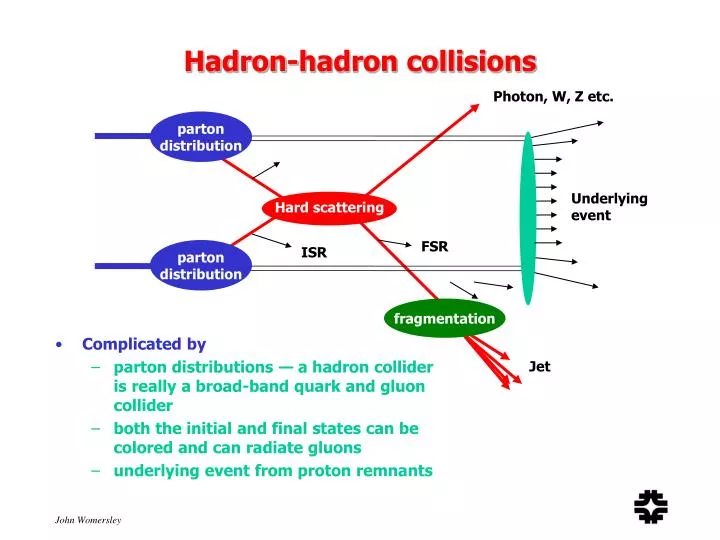
1. Hadron-hadron collisions Photon, W, Z etc. • Complicated by • parton distributions — a hadron collider is really a broad-band quark and gluon collider • both the initial and final states can be colored and can radiate gluons • underlying event from proton remnants parton distribution Underlying event Hard scattering FSR parton distribution ISR fragmentation Jet

2. Parton Distributions Sum over initial states Point Cross Section Renormalization Scale Factorization Scale Order sm

3. =0 (=90) E =–1 =1 (~40)  =2 (~15) =3 (~6) Hadron Collider variables • The incoming parton momenta x1 and x2 are unknown, and usually the beam particle remnants escape down the beam pipe • longitudinal motion of the centre of mass cannot be reconstructed • Focus on transverse variables • Transverse Energy ET = E sin  (= pT if mass = 0) • and longitudinally boost-invariant quantities • Pseudorapidity  = – log (tan /2) (= rapidity y if mass = 0) • particle production typically scales per unit rapidity

4. Quantum Chromodynamics • Gauge theory (like electromagnetism) describing fermions (quarks) which carry an SU(3) charge (color) and interact through the exchange of vector bosons (gluons) • Interesting features: • gluons are themselves colored • interactions are strong • coupling constant runs rapidly • becomes weak at momentum transfers above a few GeV

5. e e g p q q q Quarks • These features lead to a picture where quarks and gluons are bound inside hadrons if left to themselves, but behave like “free” particles if probed at high momentum transfer • this is exactly what was seen in deep inelastic scattering experiments at SLAC in the late 1960’s which led to the genesis of QCD • electron beam scattered off nucleons ina target • electron scattered from pointlike constituents inside the nucleon • ~ 1/sin4(q/2) behavior like Rutherford scattering • other (spectator) quarks donot participate

6. e e g p q q q Fragmentation So what happens to this quark that was knocked out of the proton? • s is large • lots of gluon radiation and pair production of quarks in the color field between the outgoing quark and the colored remnant of the nucleon • these quarks and gluons produced in the “wake” of the outgoing quark recombine to form a “spray” of roughly collinear, colorless hadrons: a jet • “fragmentation” or “hadronization”

7. jet Jet p g colorless states - hadrons Fragmentation process p outgoing parton Hard scatter jet What are jets? • The hadrons in a jet have small transverse momentum relative to the parent parton’s direction and the sum of their longitudinal momenta is roughly the parent parton momentum • Jets are the experimental signatures of quarks and gluons and manifest themselves as localized clusters of energy

8. e- Z0/g e+ O(as0) O(as1) O(as2) e- Z0/ Hadrons e+ Perturbative phase as<1 (Parton Level) Non-perturbative phase as1 e- e- Z0/g Z0/g e+ e+ e+e– annihilation • Fixed order QCD calculation of e+e- (Z0/g)* hadrons : • Monte Carlo approach (PYTHIA, HERWIG, etc.)

9. e+e–  +– e+e– qq e+e– qqg

10. Jet Algorithms • The goal is to be able to apply the “same” jet clustering algorithm to data and theoretical calculations without ambiguities. • Jets at the “Parton Level” • i.e., before hadronization • Fixed order QCD or (Next-to-) leading logarithmic summations to all orders Leading Order outgoing parton Hard scatter

11. Jets at the particle (hadron) level • Jets at the “detector level” The idea is to come up with a jet algorithm which minimizes the non-perturbative hadronization effects Jet hadrons fragmentation process outgoing parton Hard scatter Particle Shower Calorimeter hadrons fragmentation process outgoing parton Hard scatter

12. Jet Algorithms • Traditional Choice at hadron colliders: cone algorithms • Jet = sum of energy within R2 = 2 + 2 • Traditional choice in e+e–: successive recombination algorithms • Jet = sum of particles or cells close in relative kT Sum contents of cone Recombine

13. Theoretical requirements • Infrared safety • insensitive to “soft” radiation • Collinear safety • Low sensitivity to hadronization • Invariance under boosts • Same jets solutions independent of boost • Boundary stability • maximum ET = s/2 • Order independence • Same jets at parton/particle/detector levels • Straightforward implementation

14. Effect of pileup on Thrust kT algorithm jets, ET > 30 GeV DØ MC Experimental requirements • Detector independence • can everybody implement this? • Best resolution and smallest biases in jet energy and direction • Stability • as luminosity increases • insensitive to noise, pileup and small negative energies • Computational efficiency • Maximal reconstruction efficiency • Ease of calibration • ...

15. Splitting and Merging of Cone Jets • Jets spread out in the calorimeter, and cannot be perfectly resolved. Some compromise is necessary • Overlapping cone jets lead to ambiguous jet definitions: • which clusters belong in the jet? • do I have one or two jets? • Need to define split/merge rules: e.g. DØ choices • overlapping jets are merged if they share > 50% of the lower ET jet • otherwise they are split: each cell is assigned to the closer jet • but the process can get very involved when three or more jets overlap Merged Isolated Split “Complex” 60 GeV

16. Rsep • Ad hoc parameter introduced to mock up experimental jet separation effects in NLO theoretical calculations

17. kT algorithm

18. Does kT find the same jets?

19. kT vs. cone jets • It has been suggested that kT would give improved invariant mass reconstruction for X  multijet states • Not clear that this is true in practice: • 1000 Z bb events from DØ GEANT simulation reconstructed with C++ offline clustering and jet reconstruction Invariant mass of leading two jets (ET > 20, ||<2) Jet response corrections included R=0.7 cone jet-finder kT jet-finder

20. Jet Energy Calibration 1. Establish calorimeter stability and uniformity • pulsers, light sources • azimuthal symmetry of energy flow in collisions • muons 2. Establish the overall energy scale of the calorimeter • Testbeam data • Set E/p = 1 for isolated tracks • momentum measured using central tracker • EM resonances (0 , J/,  and Z  e+e–) • adjust calibration to obtain the known mass 3. Relate EM energy scale to jet energy scale • Monte Carlo modelling of jet fragmentation + testbeam hadrons • CDF • ET balance in jet + photon events • DØ

21. Cone Jet Energy Scale

22. Response Correction • Use pT balance in  + jet events • photon calibrated using Z  e+e– events • assume missing pT component parallel to jet is due to jet miscalibration Jet response

23. kT jet energy scale • Similar procedure, but: • no out-of-cone showering losses • can’t just use energy in a cone for the underlying event and noise, so derive this correction from Monte Carlo jets with overlaid crossings • Response:

24. Overall Energy scale correction kT jet energy scale R = 0.7 Cone R = 0.7 Cone

25. Jet Resolutions • Determined from collider data using dijet ET balance

26. Jet cross sections at s = 1.8 TeV R = 0.7 cone jets • Cross section falls by seven orders of magnitude from 50 to 450 GeV • Pretty good agreement with NLO QCD over the whole range DØ jet  0.5 0.1  jet  0.7

27. Highest ET jet event in DØ ET1 = 475 GeV, h1 = -0.69, x1=0.66 ET2 = 472 GeV, h2 = 0.69, x2=0.66 MJJ = 1.2 TeV Q2 = 2.2x105 GeV2

28. What’s happening at high ET? CDF 0.1<||<0.7 DØ ||<0.5 • So much has been said about the high-ET behaviour of the cross section that it is hard to know what can usefully be added: Figure 1: “The Horse is Dead” NB Systematic errors not plotted Figure 1: “The horse is dead”

29. The DØ and CDF data agree • DØ analyzed 0.1 <||< 0.7 to compare with CDF • Blazey and Flaugher, hep-ex/9903058 Ann. Rev. article • Studies (e.g. CTEQ4HJ distributions shown above) show that one can boost the gluon distribution at high-x without violating experimental constraints*; results are more compatible with CDF data points *except maybe fixed-target photons, which require big kT corrections before they can be made to agree with QCD (see later)

30. CDF data DØ data Jet data with latest CTEQ5 PDF’s

31. DØ inclusive cross sections up to || = 3.0 Comparison with JETRAD usingCTEQ3M,  = ETmax/2 • 0.0    0.5 • 0.5    1.0 • 1.0    1.5 • 1.5    2.0 • 2.0    3.0 d2 (dET d) (fb/GeV) • 0.0    0.5 DØ Preliminary ET (GeV) • 1.5    2.0 • 0.5    1.0 Data - Theory / Theory DØ Preliminary DØ Preliminary • 1.0    1.5 • 2.0    3.0 DØ Preliminary DØ Preliminary ET (GeV) ET (GeV) Forward Jets DØ Preliminary

32. Triple differential dijet cross section 1 Trigger Jet 0.1<|h|<0.7 Can be used to extract or constrain PDF’s Beam line 2 Probe Jet ET>10 GeV 0.1<|h|<0.7, 0.7<|h|<1.4, 1.4<|h|<2.1, 2.1<|h|<3.0 At high ET, the same behaviour as the inclusive cross section, presumably because largely the same events

33. Tevatron jet data can constrain PDF’s Tevatron HERA Fixed Target • For dijets:

34. What have we learned from all this? • Whether nature has actually exploited the “freedom” to enhance gluon distributions at large x will only be clear with the addition of more data • with 2fb-1 the reach in ET will increase by ~70 GeVand should make the asymptotic behaviour clearer • whatever the Run II data show, this has been a useful lesson: • parton distributions have uncertainties, whether made explicit or not • we should aim for a full understanding of experimental systematics and their correlations • We can then use the jet data to reduce these uncertainties on the parton distributions It’s a good thing

35. W samples

36. l q W q W W(Z) q g g q’ q’ p n (l) W and Z production at hadron colliders O(as0) Production dominated byqq annihilation (~60% valence-sea, ~20% sea-sea) Due to very large pp  jj production, need to use leptonic decays BR ~ 11% (W), ~3% (Z) per mode p q O(as) Higher order QCD corrections: • Boson produced with mean pT ~ 10 GeV • Boson + jet events (W+jet ~ 7%, ETjet > 25 GeV ) • Inclusive cross sections larger • Boson decay angular distribution modified Benefits of studying QCD with W&Z Bosons: • Distinctive event signatures • Low backgrounds • Large Q2 (Q2 ~ Mass2 ~ 6500 GeV2) • Well understood Electroweak Vertex

37. W identification • Isolated lepton + missing ET Transverse mass

38. Cross section measurements • Test O(2) QCD predictions for W/Z production • (pp  W + X) B(W  ) • (pp  Z + X) B(Z  ) • QCD in excellent agreement with data • so much so that it has been seriously suggested to use W as the absolute luminosity normalization in future Note: CDF luminosity normalization is 6.2% higher than DØ (divide CDF cross sections by 1.062 to compare with DØ)

39. W mass measurement • One of the major goals of the Tevatron program: together with mt, provides strong constraints on the SM and mH • Simplest method: • fit transverse mass distribution • Recent method: • also fit pT(lepton) and missing ET and combine the three • It’s all in the systematics • must constantly fight to keep beating them down as the statistical power of the data demands more precision • Use the Z to constrain many effects • Energy scale • pT distribution • etc etc.

40. DO 1999 measurement • Summer 2002 mW measurements: • Hadron colliders 80.454 (59) • LEP 80.450 (39) • Anticipated • With 2fb-1, mW ~ 27 MeV per experiment • With 15fb-1, mW ~ 17 MeV per experiment 95 MeV total

41. W and Z pT • Large pT (> 30 GeV) • use pQCD, O(s2) calculations exist • Small pT (< 10 GeV) • resum large logarithms of MW2/pT2 • Match the two regions and include non-perturbative parameters extracted from data to describe pT ~ QCD

42. DØ pTW measurement Preliminary Preliminary Data–Theory/Theory Arnold and Kauffman Nucl. Phys. B349, 381 (91). O(s2), b-space, MRSA’ (after detector simulation) 2/dof=7/19 (pTW<120 GeV/c) 2 /dof=10/21 (pTW<200GeV/c) • Resolution effects dominate at low pT • High pT dominated by statistics and backgrounds

43. DØ pTZ measurement • New DØ results hep-ex/9907009 Data–Theory/Theory Fixed Order NLO QCD Data–Theory/Theory Resummed Ladinsky & Yuan Ellis & Veseli and Davies, Webber & Stirling (Resummed) not quite as good a description of the data Data

44. CDF pTW and pTZ Ellis, Ross, Veseli, NP B503, 309 (97). O(s), qT space, after detector simulation. ResBos: Balasz, Yuan,PRD 56, 5558 (1997), O(s2), b-space VBP: Ellis, Veseli,NP B511,649 (1998), O(s), qT-space

45. W + jet production • A test of higher order corrections: • Calculations from DYRAD (Giele, Glover, Kosower) LO as a2s One jet or two?

46. W + jet measurements • DØ used to show a W+1jet/W+0jet ratio badly in disagreement with QCD. This is no longer shown (the data were basically correct, but there was a bug in the DØ version of the DYRAD theory program). • CDF measurement of W+jets cross section agrees well with QCD:

47. CDF W/Z + n jets • Data vs. tree-level predictions for various scale choices • These processes are of interest as the background to top, Higgs, etc.

48. Colour coherence in W + jet events Compare pattern of soft particle flow around jet to that around the W Calorimeter Tower bjet Jet bW W • In each annular region, measure number of calorimeter towers with ET > 250 MeV • Plot ratio of jet-side to W-side as a function of angle  ( = 0 is “near beam”,  =  is “far beam”) Search disks:R(inner)=0.7, R(outer)=1.5 b = tan-1(sign(hW,Jet) Df / Dh)

49. Colour coherence in W + jet events OK X Jet towers/W towers X OK Data agree with PYTHIA and MLLA+LPHD; Do not agree with models without coherence Near Beam Far Beam

50. l+ l+ l+ */Z */Z */Z l– l– l– Drell-Yan process O(as0) • Measure d/dM forpp  l+l- + X • Because leptons can be measured well, and the process is well understood, this is a sensitive test for new physics (Z’, compositeness) q q O(as) q q g q g q’