Download
1 / 30
350 likes | 560 Views
Dry and Moist Convection in the Atmosphere. General principals of convection & examples Daytime dry convective boundary layer Shallow and deep cloud convection. Convection- general principles. Driven by buoyancy – that is air is heavier or lighter than its surroundings

E N D
Dry and Moist Convection in the Atmosphere General principals of convection & examples Daytime dry convective boundary layer Shallow and deep cloud convection
Convection- general principles • Driven by buoyancy – that is air is heavier or lighter than its surroundings • Lighter air rises – heavier air sinks • Dynamically is non-hydrostatic – that is vertical equation of motion involves imbalance between pressure force and force of gravity • Buoyancy from temperature or mass difference from surroundings. • Buoyant air has potential energy that converts to kinetic energy of rising motion.
General principles-cont. • Convective motion is cellular – sometimes with some organization/pattern. • Cells consist of upward and downward branches and connecting horizontal flow. • Usually kinetic energy generated in only one branch – the active branch – other branch loses kinetic energy to potential energy – the inactive branch. • Net generation of KE to maintain against friction by active branch being narrower, i.e. distribution of vertical motion skewed (w’**3) toward direction of active generation
Buoyancy • The quantity r’ g / r0 is the vertical acceleration of air per unit mass due to its density being different than that of its surroundings – this is referred to as the buoyancy. Density varies either because of variation of temperature or humidity or liquid water– the first two can be lumped together using the concept of virtual temperature. Another such idea for liquid water.
Radiative drivers of buoyancy/convection • Daytime surface heating – some goes into heating air – drives large convection cells that are the dominant component of the daytime boundary layer – leading to rapid mixing of air over this layer. • Cloud top cooling – air at top of clouds
Vertical equation of motion is: r dw/dt=-r g – dp/dz Acceleration = sinking by gravity + push by pressure from high to low. Assume dry air. Subtract basic state from p and r. r’ = r - r0(z), p’ = p - p0 (z) , where dp0/dz = -r0 g (hydrostatic balance), The term dp’/dz is only important for acoustic waves. For boundary layer convection use: r0dw/dt =-r’ g, • Heating directly changes temperature. Use gas law to get density in terms of T– i.e. T’/T0 = - r’ / r0 • Where moisture aggects density, include through “virtual temperature” Tv, i.e. the temperature that would give the density for dry air
Daytime dry convective boundary layer • Net radiative heating at surface warms air and drives convection have near adiabatic lapse rate and near uniform water vapor (constant virtual potential temperature). • For uniform mixing, can use vertical averages as state variables – temperature and column water vapor content. • Sources are at boundaries. Also need height of this layer. Heat added at surface can either increase temperature or raise the height of BL –both happen.
Daytime boundary layer entrainment • At top of daytime boundary layer, have an interface with stable air. • Overlying stable air is warmer (i.e. higher potential temperature) and dryer than air in boundary layer. • The mixing at this interface “entrains”, i.e. pulls in, this warm dry air acting as a source of heating and removal of humidity for the boundary layer average values. • Depth incresases over day.
Contrast – nighttime boundary layer • At night, mixing only extends up to MO scale L, air stable above • MO theory matches into a temperature inversion for O (100m) vertical scale. • Above this inversion, have at night residual layer that is nearly adiabatic – what remains of daytime slowly coling by radiation.
Structure and diurnal growth of the CBL , u, v are well mixed through the CBL. Thus the CBL can be treated as a single layer of air with changing depth.
An example of entrainment (Ciesielski et al. 1995) Entrainment velocity, we: Several approaches, still is an area of active research. • We=dzi/dt, typically 0.01 to 0.2 m/s, can be 1m/s. • In case of free convection: Entrainment of free atmosphere
Entrainment layer: • Entrainment layer (EL): refers to stable air at the top of the ML, consists of free atmosphere downward and overshooting thermals upward. is negative. • The thickness of the entrainment layer varies proportionally with the depth of the convective mixed layer, h/ho=0.21+1.31(Ri*)-1 Where Ri* is Richardson number • EL is critical for tracer exchange between ABL and free atmosphere. Free atmosphere Growing ABL
Key Atmospheric Boundary Layer Scales Friction velocity u* =sqrt[-u’w’] Surface shear zone length scale: z ABL height: zi Convective velocity w* = (g zi[w’ T’v/ T0] )1/3 Shear velocity in surface layer: U = u* / k, k = 0.4 Shear zone depth scale L = depth over which turbulence is predominantly generated by shear
Bulk Boundary Layers: • Bulk boundary layer refers to case where only know average properties of a layer not values at a level: Could be model’s lowest layer is too thick to be treated as a level or could be you want to treat average values over the whole BL Use { }ab to denote averages between levels a and b: Then: {U}ab = u* {F} ab, where F = U/u* as obtained from MOS theory, i.e. F = (log(z/z0) – y(z)) /k . We can use the formalism of a drag coefficient Cd = 1./ {F}ab2 to get momentum flux u*2 from the layer winds. This can only work if the MOS applies throughout the layer
Bulk formalism applied to whole BL • MOS can be made to work throughout a convective BL, but not directly for stable BL. • Winds: how does log (z/z0) – y(z) vary with z? Since the latter term disappears with large z , we may expect that the contribution is from primarily the log term: for an oceanic value z0 is about 1 mm the z/z0 is varying from say 104 at 10 m to 106 at 1km, and it is close to the latter most of the time. This makes the log term vary from 9.2 to 13.8 and it is close to the latter over most of the averaging interval. There is some height zeff that is approximately half of the BL height that plugged into the log will give its average over the interval. Just using the BK height in the log term may be good enough. The resulting drag coefficient will be smaller than the more often found 10 m value, maybe reduced for the ocean from 1.4 10-3 to 1.0 10-3
Conceptual model of CBL(Lilly 1968):Because u, and q are well mixed in a CBL, we can treat them as constants relative to height within the CBL. we e h qT Cloud layer
u Air Entrainment (t+dt)- (t)=h+h) Tennekes 1973
, u, v
Objective of cloud convection lectures • Clouds are horribly complicated even without thinking about turbulence. • Turbulence is horribly complicated • Atmospheric radiation is horribly complicated • Clouds are very important because of their impacts on climate system and their transport of water vapor and other atmospheric constituents • What clouds do is largely through their turbulence (and radiative interactions). • To work with clouds, we must know all (not very many) the simple things that can be said about them. .
Shallow Cumulus and Deep Cumulus Tropical and semitropical moist oceanic boundary layers without an overlying stratiform cloud layer typically have relative humidities of about 75% and humidity drops off about 2% per 100m in the BL so require a temperature increase of about 4-5C (adiabatic uplift to about 400-500 m) to reach saturation – (a little higher than if the humidity were perfectly mixed as we often assume). The lapse rate follows near a moist adiabat up to about 1.5 km and above that is generally an inversion layer of 1-2km thick where on average the lapse rate is 0.5 to 1K/km less than moist adiabatic. Above there to near the tropopause, the lapse rate becomes steeper than moist adiabatic. From the LCL to the inversion, air mixed up from below saturates and so must form either stratified or cumulus. For some combination of warmer ocean surface, and higher inversion layer, cumulus is a more stable configuration.
Characterization of cumulus clouds in terms of Mc What’s good? • Simple • Captures much of what cloud does for transport of energy water and other constituents. What’s bad? • Lacks information as to cloud area, thus provides almost no information related to radiative properties. • Lacks information as to vertical velocities in the cloud, thus provides very limited information for cloud physics. • Does not say how clouds start and stop- it is a steady state view. • Not obvious how to link to any turbulence modeling.
Modeling the Convection • The mass flux plume model needs only two rules to be applied: • what is the initial mass flux at cloud base? • how does the mass flux change with altitude? • Part of this latter question is how high does the convection extend. The change with altitude is modeled as a buoyant plume. There have been many versions of how to do such plumes but they all contain similar elements. The plume must be started with a certain buoyancy. It moves upward as long as it retains buoyancy. How far it overshoots into the overlying region of negative buoyancy depends on how much kinetic energy it may have gained.
Entrainment and Detrainment Entrainment for a plume model describes the rate at which external air is added to the convecting plume per unit rise of the plume; that is (dMc/dz)entrainment = e Mc, where e is the entrainment parameter. Detrainment is the rate at which plume air is lost to the outside atmosphere: (dMc/dz)detrainment = -d Mc. The sum of these two effects is: dMc/dz = (e-d) Mc These expressions alone do not show how to distinguish when both are happening. We need an other expression showing how a conserved quantity q is affected by entrainment of outside air and detrainment of air inside cloud. d/dz (Mc qc) = (e[q]- d qc )Mc ; This combines with above: dqc/dz =e ([q]-qc)
How to know rates of entrainment and detrainment? These rates are determined by analysis of observations and LES models. As just shown, the degree to which a tracer in the cloud is being mixed with outside air as a function of height gives the entrainment. Change of mass flux with height then gives the detrainment. Observations of these indicate large rates of entrainment and even larger detrainment in the shallow cumulus layer & then near constant Mc until the upper troposphere where the deep cumulus have large detrainment. Detrainment is a result of air losing its buoyancy. This happens through some combination of: a complete plume stopped because its buoyacy becomes negative; b) mixing of entraining air with some of the resulting mixture becoming negatively buoyant. The detrained air does one of two things depending on its stability: a) if stable, sinks to level of neutral buoyancy and spreads out laterally; b) if unstable, continues to sink as a downward convective plume.
Properties of tophat cumulus model How do we do turbulent transports with the tophat model? If q is any conservative quantity such as total water (for no rain). [w’q’] = Mc qc - Mc [q] Effect of large scale is d[q]/dt = -d/dz[w’q’]. With the tophat model (and small a approximation) this equals: -d/dz[w’q’] = Mc d×[qc-q] - Mc d[q]/dz This can be derived from a) direct conservation argument b) slogging through the algebra from the above definition and definitions of entrainment and detrainment. The only piece worth remembering is the direct argument, but I also do b) to convince you the equations make sense.
Derivation of cumulus convection effect on area average fields The direct argument is that anything happening only in the cloud is not contributing to an average over a large area outside because of the clouds smallness. Thus, convection only affects [q] by sinking external to the cloud acting on its gradient or by the air from in the cloud being mixed into outside air through detrainment. For the more tedious derivation, we use the previously derived expressions: dMc/dz = (e–d) Mc,, d/dz(Mcqc) = (e[q]-dqc) Mc d/dz[w’q’] = d(Mcqc)/dz – [q] dMc/dz -Mc d[q]/dz = (e [q]-d qc )Mc– [q] Mc (e-d) - LSF = d ([q]- qc) -LSF
Cumulus production of warming and drying At levels where there is no detrainment we see that the effect of cumulus upward transport is only through its return circulation outside the cloud to carry downward the mean quantity transported. Thus for moisture and transport moisture this goives what may seem paradoxical at first, only to produce a warming and a drying from subsidence. Of course the integral of these has to equal the heating and moisture loss for net condensation of water vapor. Thus what the model is really doing is telling us how to use the vertical profiles of Mc,dMc/dz and qc-[q] give the effect at any level of the cumulus on the large scale environment.
Coupling of Convective Mixed Layer Temperatures to Surface Fluxes For large z , the MOS gradient function for dT/dz is proportional to z-1/3. That is: fH(z) = 0.7 k/34z-1/3 to be used with: dT/dz = (T*/kz) fH(z) Also recall: z = [w’T’/Tv] /u*3, T* = [w’T’]/u* so the friction velocities cancel in the factor T* z-1/3 and we have the temperature gradient proportional to heat flux to the 2/3 power and z-1/3 . We can integrate to get T in terms of heat flux or vice versa. T = 0.7 Tv1/3 [w’T’]2/3 / (gz)1/3 We can put zi in this by averaging over the mixed layer and picking up a factor of 3/2 . .
Turbulence model – continued From our previous derivations, we know that turbulent energy is generated by momentum transport down a shear gradient so that: generation = K (dU/dz)2 The dissipation consists of buoyancy dissipation and frictional dissipation. The buoyancy dissipation derives from downward temperature transport: buoyancy dissipation = (K g / [Tv] ) d[Tv]/dz; Also remember: Ri = buoyancy dissipation/generation Our objective is to get physically plausible relations that match what we already know in the surface layer. We model the eddy diffusion coefficients :K = a sqrt(e /[u’w’]) Kdef , where Kdef = [u’w’] / dU/dz = sqrt(u’w’) lm, where lm is the momentum mixing length lm = sqrt [u’w’] / dU/dz. And the adjustable constant “a” = sqrt ( [u’w’]/e) as observed in the surface mixed layer. With this K is made to fit the surface layer theory and elsewhere is: K = lm sqrt(e)