Download
1 / 33
340 likes | 564 Views
Software Engineering. Chapter Ten Software Project Management. Learning Outcomes Be able to choose a cost estimation technique for a software project Be able to estimate the size of a software project based on its requirements specification

E N D
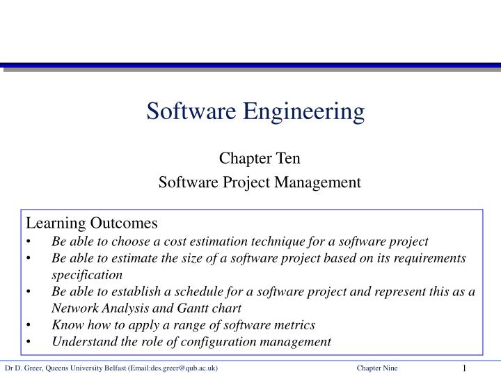
Software Engineering Chapter Ten Software Project Management • Learning Outcomes • Be able to choose a cost estimation technique for a software project • Be able to estimate the size of a software project based on its requirements specification • Be able to establish a schedule for a software project and represent this as a Network Analysis and Gantt chart • Know how to apply a range of software metrics • Understand the role of configuration management
Cost Estimation Techniques • Expert Judgement • Past Experience • Build up a databank of past projects and their cost • Top down • Break the problem up into smaller problems and estimate these • Function Point Analysis • Uses the requirements specification to assess inputs, outputs, file accesses, user interactions and interfaces and calculates the size based on these • Algorithmic Cost Modelling • Main technique is COnstructive COst Modelling (COCOMO)
Function Point Analysis • Based on a combination of program characteristics • external inputs (I) • external outputs (O) • user interactions/ enquiries e.g. menu selection, queries.. (E) • logical files used by the system (L) • external interfaces to other applications (F) • A weight is associated with each of these
Function points - example • UFP = number of Unadjusted Function Points • Average level: UFP = 4I + 5O + 4E + 10L + 7F • Simple I&O, average E&L, Complex F: UFP = 3I + 4O + 4E + 10L + 10F • UFP is then adjusted to take account of the type of application • This adjustment is made by multiplying by a factor TCF, (Technical Complexity Factor) • 14 characteristics are scored from 0 (no influence) to 6 (strong influence): • data communications, distributed functions, performance, transaction rate, facilitate change, etc.. • TCF = 0.65 + 0.01DI • where DI = the total degree of influence
Function points - example • Number of function points FP = UFP * TCF • FPs can be used to estimate LOC depending on the average number of LOC per FP for a given language e.g. 1fp = 106 lines of COBOL,128 of C, 64 of C++, 32 of VB • Problems: • FPs very subjective - cannot be counted automatically • only 3 complexity levels • need for calibration
Algorithmic cost modelling • Cost is estimated as a mathematical function of product, project and process attributes • The function is derived from a study of historical costing data • Most commonly used product attribute for cost estimation is LOC (code size) • Most models are basically similar but with different attribute values • COCOMO - Constructive Cost Model • Exists in three stages • Basic - Gives a 'ball-park' estimate based on product attributes • Intermediate - modifies basic estimate using project and process attributes • Advanced - Estimates project phases and parts separately
COCOMO • 3 classes of project • Organic mode small teams, familiar environment, well-understood applications, no difficult non-functional requirements • Semi-detached mode Project team may have experience mixture, system may have more significant non-functional constraints, organisation may have less familiarity with application • Embedded Hardware/software systems, tight constraints, unusual for team to have deep application experience • Formula: E = a (KDSI) b, D = 2.5(E)c • E = Effort in Person-months • a ,b & c are constants based on project class & historical data • D = development time • KDSI = Thousands of Delivered Source Instructions (~Lines of Code)
COCOMO Class a b c Organic 2.4 1.05 0.38 Semi-detached 3.0 1.12 0.35 Embedded 3.6 1.30 0.32 Example: Organic mode: 42,000 delivered source instructions E = 2.4 * 42 1.05 = 121.5 person months D = 2.5 * 121.5 0.38 = 15.5 months No. Personnel = E/D = 7.8
Intermediate COCOMO • Takes basic COCOMO as starting point • Identifies personnel, product, computer and project attributes which affect cost • Multiplies basic cost by attribute multipliers 1. Product attributes • Required software reliability (RELY) • Database Size (DATA) • Product Complexity (CPLX) 2. Computer Attributes • Execution time constraints (TIME) • Storage constraints (STOR) • Virtual machine volatility (VIRT) • Computer turnaround time (TURN)
3. Personnel Attributes • Analyst capability (ACAP) • Programmer capability (PCAP) • Applications experience (AEXP) • Virtual machine Experience (VEXP) • Programming language experience (LEXP) 4. Project Attributes • Modern programming practices (MODP) • Software Tools (TOOL) • Required Development schedule (SCED) • These are attributes which were found to be significant in one organisation with a limited size of project history database • Other attributes may be more significant for other projects
Example • Embedded software system on microcomputer hardware. • Basic COCOMO predicts a 45 person-month effort requirement • Attributes = RELY (1.15), STOR (1.21), TIME (1.10), TOOL (1.10) • Intermediate COCOMO predicts • 45 * 1.15 * 1.21 * 1.1 * 1.1 = 75.8 person months • Total cost = say £3000 per month = £227,302 • Alternative 1: Use a faster CPU and more memory to reduce TIME and STOR attribute multipliers • Alternative 2: Buy some CASE tools
Alternative 1: Faster Machine • Processor capacity and store doubled • TIME and STOR multipliers = 1 • RELY still 1.15 • Say, Fewer tools available • TOOL = 1.15 • Extra investment of £30, 000 required • Total cost = 45 * 1.15 * 1.15 = 59.5 Person-months = £178,538 + 30,000 = £208,538 • Cost saving = 227,302 – 208538 = 18,764
Alternative 2: CASE • Additional CASE tool cost of £15,000 • Reduces TIME (1), tool multipliers(1) • Increases experience multiplier to 1.1 • RELY still 1.15, STOR still 1.21 • Cost = 45 * 1.15 * 1.21 * 1.1 = 68.9 person months • = £206,638 • Total Cost = £15,000 + £206,638 = 221,638 • Cost Saving = 227,302 - 221,638 = £5,664 • ALTERNATIVE 1 is best
Project Scheduling • Work Breakdown Structures • Divide the project up into tasks OnLine Frequent Flyer Points Obtain Funding Client Side Code Implement Database Screen Designs Validation Linking to Server Side Main Applet Authorisation Code Account Balance System Testing Calculate Account Balance Display Account Balance Release
OnLine Frequent Flyer Points Obtain Funding Set Up Team Client Side Code Implement Database Screen Designs Validation Linking to Server Side Main Applet Authorisation Code Account Balance System Testing Calculate Account Balance Display Account Balance Release
0 0 0 Start 0 0 0 Network Analysis - durations 13 ES D EF 5 H Start 3 5 E LS F LF L B 10 15 21 F C K 5 15 A G 10 12 7 D J I
ES 0 D 0 EF 0 Start Start LS 0 0 F LF 0 Network Analysis – ES & EF 10 13 23 5 H 3 5 5 10 E L B 10 10 15 25 21 F C K 0 5 5 15 A G EF=ES+D ES is the latest EF of a tasks predecessors 5 10 15 12 7 D J I
0 0 0 Start 0 0 0 Network Analysis – ES & EF 10 13 23 ES D EF 25 5 30 H Start 75 3 78 5 5 10 E LS F LF L B 25 10 35 10 15 25 54 21 75 F C K 0 5 5 15 15 30 A G 5 10 15 42 12 54 35 7 42 D J I
0 0 0 Start 0 0 0 Network Analysis – LS & LF 10 13 23 ES D EF 25 5 30 H Start 75 3 78 5 5 10 E 22 35 LS F LF L B 30 35 75 78 5 10 25 10 35 10 15 25 54 21 75 F C K 25 35 10 25 0 5 5 54 75 15 15 30 A G 0 5 20 35 LF=earliest LS of next tasks 5 10 15 42 12 54 35 7 42 D J I 10 20 42 54 35 42
0 0 0 Start 0 0 0 Network Analysis –Float & Critical Path 10 13 23 ES D EF 25 5 30 H Start 75 3 78 5 5 10 E 22 12 35 LS F LF L B 30 5 35 75 0 78 5 0 10 25 10 35 10 15 25 54 21 75 F C K 25 0 35 10 0 25 0 5 5 54 0 75 15 15 30 A G 0 0 5 20 5 35 F=LF-EF Critical Path = shortest path to finish the project 5 10 15 42 12 54 35 7 42 D J I 10 5 20 42 0 54 35 0 42
Configuration management • All products of the software process may have to be managed • Specifications • Designs • Programs • Test data • User manuals • Thousands of separate documents are generated for a large software system • CM Plan • Defines the types of documents to be managed and a document naming scheme • Defines who takes responsibility for the CM procedures and creation of baselines • Defines policies for change control and version management • Defines the CM records which must be maintained
The configuration database • All CM information should be maintained in a configuration database • allow queries • Who has a particular system version? • What platform is required for a particular version? • What versions are affected by a change to component X? • How many reported faults in version T? • The CM database should preferably be linked to the software being managed • When a programmer downloads a program it is ‘booked’ out to him/her • Could be linked to a CASE tool
Derivation history • Record of changes applied to a document or code component • Should record, in outline, the change made, the rationale for the change, who made the change and when it was implemented • May be included as a comment in code. If a standard prologue style is used for the derivation history, tools can process this automatically /*********************************************************** /* ID Modified By Date Reason /* TC01 S Smith 1 Dec 02 Update to Tax /* Rules /* TC02 J Bloggs 10 Dec 02 Fix x bug in /* price calc
Versions/variants/releases • Version An instance of a system which is functionally distinct in some way from other system instances • Variant An instance of a system which is functionally identical but non-functionally distinct from other instances of a system • Release An instance of a system which is distributed to users outside of the development team • Version Numbering • Simple naming scheme uses a linear derivation e.g. V1, V1.1, V1.2, V2.1, V2.2 etc. • Better way is Attribute Naming • Examples of attributes are Date, Creator, Programming Language, Customer, Status etc • AC3D (language =Java, platform = NT4, date = Jan 1999)
Software Metrics • “When you can measure what you are speaking about and express it in numbers, you know something about it” (Kelvin) • Allow processes and products to be assessed • Used as indicators for improvement • Size-oriented Metrics • Lines of Code (LOC) • Effort (Person-Months) • Cost (£) • Pages of Documentation • Numbers of Errors • Errors per KLOC • Cost per KLOC • Errors per person-month
Quality Metrics • Defect Removal Efficiency • DRE = E/(E+D) • E = No. Errors, before delivery • D = No. Defects after delivery • Measures how good you are at quality assurance • Defects per KLOC • C = No. Defects/ KLOC • defect = lack of conformance to a requuirement • Measures correctness • Integrity • A systems ability to withstand attacks (incl. Accidental) to its security • I = [(1-threat) x (1- security) • threat = probability that an attack will occur at a given time • security = probability that an attack will be repelled DRE should be 1
Design Complexity • 'fan-in and fan-out' in a structure chart. • High fan-in (number of calling functions) = high coupling • High fan-out (number of calls) = high coupling (complexity). • Complexity = Length * (Fan-in * Fan-out)2 (Henry & Kafura, 1990) (Length is any measure of program size such as LOC) • Other metrics include • Cyclomatic complexity. The complexity of program control • Length of identifiers • Depth of conditional nesting • Gunnings Fog index (based on length of sentences/ no. of syllables) • Reliability metrics - next
Reliability Metrics • Probability of failure on demand • This is a measure of the likelihood that the system will fail when a service request is made • POFOD = 0.001 means 1 out of 1000 service requests result in failure • Relevant for safety-critical or non-stop systems • Computed by measuring the number of system failures for a given number of system inputs • Rate of fault occurrence (ROCOF) • Frequency of occurrence of unexpected behaviour • ROCOF of 0.02 means 2 failures are likely in each 100 operational time units • Relevant for operating systems, transaction processing systems • Computed by measuring the time (or number of transactions) between system failures
Reliability Metrics • Mean time to failure • Measure of the time between observed failures • MTTF of 500 means that the time between failures is 500 time units • Computed by measuring the time (or number of transactions) between system failures • Mean time to Repair (MTTR) • average time to correct a failure • Computed by measuring the time from the failure occurs to the time it is repaired • Availability • Measure of how likely the system is available for use. Takes repair/restart time into account • AVAIL = MTTF / MTTF + MTTR