Download
1 / 20
200 likes | 322 Views
CSE332: Data Abstractions Lecture 14: Beyond Comparison Sorting. Dan Grossman Spring 2012. The Big Picture. Surprising amount of juicy computer science: 2-3 lectures…. Simple algorithms: O( n 2 ). Fancier algorithms: O( n log n ). Comparison lower bound: ( n log n ).

E N D
CSE332: Data AbstractionsLecture 14: Beyond Comparison Sorting Dan Grossman Spring 2012
The Big Picture Surprising amount of juicy computer science: 2-3 lectures… Simple algorithms: O(n2) Fancier algorithms: O(n log n) Comparison lower bound: (n log n) Specialized algorithms: O(n) Handling huge data sets Insertion sort Selection sort Shell sort … Heap sort Merge sort Quick sort (avg) … Bucket sort Radix sort External sorting CSE332: Data Abstractions
How Fast Can We Sort? • Heap sort & Merge sort have O(nlogn) worst-case running time • Quick sort has O(nlogn) average-case running time • These bounds are all tight, actually (nlogn) • So maybe we need to dream up another algorithm with a lower asymptotic complexity, such as O(n) or O(nlog logn) • Instead: prove that this is impossible • Assuming our comparison model: The only operation an algorithm can perform on data items is a 2-element comparison CSE332: Data Abstractions
A General View of Sorting • Assume we have n elements to sort • For simplicity, assume none are equal (no duplicates) • How many permutationsof the elements (possible orderings)? • Example, n=3 a[0]<a[1]<a[2] a[0]<a[2]<a[1] a[1]<a[0]<a[2] a[1]<a[2]<a[0] a[2]<a[0]<a[1] a[2]<a[1]<a[0] • In general, n choices for least element, n-1 for next, n-2 for next, … • n(n-1)(n-2)…(2)(1) = n! possible orderings CSE332: Data Abstractions
Counting Comparisons • So every sorting algorithm has to “find” the right answer among the n! possible answers • Starts “knowing nothing” and gains information with each comparison • Intuition: Each comparison can at besteliminate half the remaining possibilities • Must narrow answer down to a single possibility • What we will show: Any sorting algorithm must do at least(1/2)nlog2 n – (1/2)n (which is (nlogn)) comparisons • Otherwise there are at least two permutations among the n! possible that cannot yet be distinguished, so the algorithm would have to guess and could be wrong CSE332: Data Abstractions
Counting Comparisons • Don’t know what the algorithm is, but it cannot make progress without doing comparisons • Eventually does a first comparison “is a < b ?" • Can use the result to decide what second comparison to do • Etc.: comparison k can be chosen based on first k-1 results • Can represent this process as a decision tree • Nodes contain “set of remaining possibilities” • Edges are “answers from a comparison” • The algorithm does not actually build the tree; it’s what our proof uses to represent “the most the algorithm could know so far” as the algorithm progresses CSE332: Data Abstractions
One Decision Tree for n=3 a < b < c, b < c < a, a < c < b, c < a < b, b < a < c, c < b < a a > b a < b a < b < c a < c < b c < a < b b < a < c b < c < a c < b < a b < c b > c a < c a > c b < a < c b < c < a c < b < a a < b < c a < c < b c < a < b c < a c > a b < c b > c b < c < a b < a < c a < c < b a < b < c • The leaves contain all the possible orderings of a, b, c • A different algorithm would lead to a different tree CSE332: Data Abstractions
Example if a < c < b possible orders a < b < c, b < c < a, a < c < b, c < a < b, b < a < c, c < b < a a > b a < b a < b < c a < c < b c < a < b b < a < c b < c < a c < b < a b < c b > c a < c a > c b < a < c b < c < a c < b < a a < b < c a < c < b c < a < b c < a c > a b < c b > c b < c < a b < a < c a < c < b a < b < c actual order CSE332: Data Abstractions
What the Decision Tree Tells Us • A binary tree because each comparison has 2 outcomes • (No duplicate elements) • (Would have 1 outcome if a comparison is redundant) • Because any data is possible, any algorithm needs to ask enough questions to produce all n! answers • Each answer is a different leaf • So the tree must be big enough to have n! leaves • Running any algorithm on any input will at best correspond to a root-to-leaf path in somedecision tree with n! leaves • So no algorithm can have worst-case running time better than the height of a tree with n! leaves • Worst-case number-of-comparisons for an algorithm is an input leading to a longest path in algorithm’s decision tree CSE332: Data Abstractions
Where are we • Proven: No comparison sort can have worst-case running time better than the height of a binary tree with n! leaves • Turns out average-case is same asymptotically • A comparison sort could be worse than this height, but it cannot be better • Now: a binary tree with n! leaves has height (nlogn) • Factorial function grows very quickly • Height could be more, but cannot be less • Conclusion: Comparison sorting is (nlogn) • An amazing computer-science result: proves all the clever programming in the world cannot sort in linear time CSE332: Data Abstractions
Lower bound on height • The height of a binary tree with L leaves is at least log2L • So the height of our decision tree, h: hlog2 (n!) property of binary trees = log2(n*(n-1)*(n-2)…(2)(1)) definition of factorial = log2n + log2(n-1) + … + log21 property of logarithms log2n + log2(n-1) + … + log2(n/2) drop smaller terms (0) log2(n/2)+ log2(n/2) + … + log2(n/2) shrink terms to log2(n/2) = (n/2)log2(n/2) arithmetic = (n/2)(log2n -log22) property of logarithms = (1/2)nlog2n – (1/2)narithmetic “=“ (nlogn) CSE332: Data Abstractions
The Big Picture Surprising amount of juicy computer science: 2-3 lectures… Simple algorithms: O(n2) Fancier algorithms: O(n log n) Comparison lower bound: (n log n) Specialized algorithms: O(n) Handling huge data sets Insertion sort Selection sort Shell sort … Heap sort Merge sort Quick sort (avg) … Bucket sort Radix sort External sorting • huh??? • Change the model – assume • more than items can be • compared! CSE332: Data Abstractions
BucketSort (a.k.a. BinSort) • If all values to be sorted are known to be integers between 1 and K (or any small range) • Create an array of size K • Put each element in its proper bucket (a.k.a. bin) • If data is only integers, no need to store more than a count of how times that bucket has been used • Output result via linear pass through array of buckets • Example: • K=5 • input (5,1,3,4,3,2,1,1,5,4,5) • output: 1,1,1,2,3,3,4,4,5,5,5 CSE332: Data Abstractions
Analyzing Bucket Sort • Overall: O(n+K) • Linear in n, but also linear in K • (nlogn) lower bound does not apply because this is not a comparison sort • Good when Kis smaller (or not much larger) than n • Do not spend time doing comparisons of duplicates • Bad when K is much larger than n • Wasted space; wasted time during final linear O(K) pass • For data in addition to integer keys, use list at each bucket CSE332: Data Abstractions
Radix sort • Radix = “the base of a number system” • Examples will use 10 because we are used to that • In implementations use larger numbers • For example, for ASCII strings, might use 128 • Idea: • Bucket sort on one digit at a time • Number of buckets = radix • Starting with least significant digit • Keeping sort stable • Invariant: After k passes (digits), the last k digits are sorted • Aside: Origins go back to the 1890 U.S. census CSE332: Data Abstractions
Example Radix = 10 Input: 478 537 9 721 3 38 143 67 0 1 2 3 4 5 6 7 8 9 721 3 143 537 67 478 38 9 Order now: 721 3 143 537 67 478 38 9 • First pass: • bucket sort by ones digit CSE332: Data Abstractions
0 1 2 3 4 5 6 7 8 9 Example 721 3 143 537 67 478 38 9 Radix = 10 0 1 2 3 4 5 6 7 8 9 3 9 721 537 38 143 67 478 Order was: 721 3 143 537 67 478 38 9 Order now: 3 9 721 537 38 143 67 478 • Second pass: • stable bucket sort by tens digit CSE332: Data Abstractions
0 1 2 3 4 5 6 7 8 9 Example 3 9 721 537 38 143 67 478 Radix = 10 0 1 2 3 4 5 6 7 8 9 3 9 38 67 143 478 537 721 Order was: 3 9 721 537 38 143 67 478 Order now: 3 9 38 67 143 478 537 721 • Third pass: • stable bucket sort by 100s digit CSE332: Data Abstractions
Analysis Input size: n Number of buckets = Radix: B Number of passes = “Digits”: P Work per pass is 1 bucket sort: O(B+n) Total work is O(P(B+n)) Compared to comparison sorts, sometimes a win, but often not • Example: Strings of English letters up to length 15 • 15*(52 + n) • This is less than n log n only if n > 33,000 • Of course, cross-over point depends on constant factors of the implementations • And radix sort can have poor locality properties CSE332: Data Abstractions
Last Slide on Sorting • Simple O(n2) sorts can be fastest for small n • Selection sort, Insertion sort (latter linear for mostly-sorted) • Good for “below a cut-off” to help divide-and-conquer sorts • O(n log n) sorts • Heap sort, in-place but not stable nor parallelizable • Merge sort, not in place but stable and works as external sort • Quick sort, in place but not stable and O(n2) in worst-case • Often fastest, but depends on costs of comparisons/copies • (nlogn)is worst-case and average lower-bound for sorting by comparisons • Non-comparison sorts • Bucket sort good for small number of key values • Radix sort uses fewer buckets and more phases • Best way to sort? It depends! CSE332: Data Abstractions