Download
1 / 62
630 likes | 672 Views
Join us for an engaging workshop series providing an introduction to MATLAB and Simulink. Covering basic syntax, linear algebra, graphing, system solving, ODEs, functions, and more. Experience hands-on learning sessions to enhance your skills!

E N D
Introduction to MATLAB and Simulink CFSEAS Workshop George Washington University Prepared by: Farhad Goodarzi
Outline • Section I (September 21st, 2019) • Background • Basic Syntax and Commands • Linear Algebra • Loops • Section II (September 28th, 2019) • Graphing & Plots • Scripts and Functions • Section III (October 5th, 2019) • Linear & System of Equations Solving • ODE Solving • Section IV (October 12th, 2019) • Functions & Call-Backs • Numerical Simulation Example for a Dynamical System • Section IV (October 26th, 2019) • Simulink
Background • MATLAB = Matrix Laboratory (developed by The MathWorks). • Opening MATLAB Working Path Command History Command Window Working Memory
Variables • Have not to be previously declared • Variable names can contain up to 63characters • Variable names must start with a letter followed by letters, digits, and underscores( Valid: x1 = 5, Invalid: 1x= 5) • Variable names are case sensitive (a1 does NOT equal A1) Operators • EX: Using command window • >> x = 5; % this is used as a comment • >> y = 3; • >> z = x + y z = 8 • Semicolon (;) : Suppresses output • Percentage (%) : Commenting. Only good for that line
MATLAB Matrices • MATLAB treats all variables as matrices. For our purposes a matrix can be thought of as an array, in fact, that is how it is stored. • Vectors are special forms of matrices and contain only one row OR one column. • Scalars are matrices with only one row AND one column
MATLAB Matrices • A matrix with only one row is called a row vector. A row vector can be created in MATLAB as follows (note the commas): » rowvec = [12 , 14 , 63] rowvec= 12 14 63 • A matrix with only one column is called a column vector. A column vector can be created in MATLAB as follows (note the semicolons): » colvec= [13 ; 45; -2] colvec= 13 45 -2
MATLAB Matrices • A matrix can be created in MATLAB as follows (note the commas AND semicolons): » matrix = [1 , 2 , 3 ; 4 , 5 ,6 ; 7 , 8 , 9] matrix = 1 2 3 4 5 6 7 8 9
Index • MATLAB index starts with 1, NOT 0! • Vector Index: • a = [22 17 7 4 42] • a(1) = 22 • a(3) = 7 • Matrix Index: • a = [7 12 42; 5 1 23; 4 9 10]; • a(1, 3) = 42 • a(3, 2) = 9
Dot Operator • For scalar operations, nothing new is needed. Example: a = 5;b = 3; ==> c = a*b %c = 15 • For element operations, a dot must be used before the operator. • Note: Dot operator not the same as dot product! • Example: • a = [1 2 3 4]; • b = [5 6 7 8]; • c = a*b • Result: ??? Error using ==> mtimes inner matrix dimensions must agree • Now, try: • c = a.*b%notice the dot! • Result: c=[5 12 21 32] • Notice what it is doing: a(1)*b(1), a(2)*b(2), etc.
Dot Product Vector Products Consider & generate two random 3*1 vectors, A & B A=rand(3,1) , B=rand(3,1) Cross Product • Check Dimensions • A*B • A*B’ • A’*B • Use MATLAB command >> C=dot(A,B) • By definition • Use MATLAB command >> C=cross(A,B) • A(2)*B(3)-A(3)*B(2) • A(3)*B(1)-A(1)*B(3) • A(1)*B(2)-A(2)*B(1)
Loops • Loop statements do not need parenthesis. The statements are recognized via tabs. • 3 general types of loops: • If/else/elseif loops • For loops • While loops • There is a 4th type, called nested loop, that can be any of the above 3 (and any combinations of them).
If/else/elseif Loops • The condition must be previously defined!
For Loops • Counter variable does not have to be i; it can be any variable • Iterations can be tightly controlled with min:stepsize:max. • No need to pre-define the counter because you are declaring in the for loop itself! for i=1:10 statement end
While Loops • As long as output of condition is a logic true, it will continue looping until the condition becomes false. • BE CAREFUL OF INFINITE LOOPS. while condition statement end
Nested Loops • Can use a mix of the different types of loops. • Very useful for performing algorithm/operations on vectors and matrices.
Examples • Write a code to print out integer numbers from 5 to 36 • Write a code to print out integers between 45 to 109 which are divisible to 3 • Write a code to print out integers between 45 to 109 which are divisible to 5 • Write a code : • If n is divisible to 3 print “divisible to 3” • elseIfn is divisible to 5 print “divisible to 5” • Elseif n is divisible by 5 and 3 print “divisible by 15”
Plots • plot –plot(x,y,linespec) • x and y vectors must be same length! • subplot –subplot(m,n,p) where mxn matrix, p = current graph • figure –creates new window for graph • title –creates text label at top of graph • xlabel/ylabel–horizontal and vertical labels for graph
Example • x=0:pi/100:2*pi; • y=sin(x); • figure; • plot(x,y) • xlabel • ylabel • title • figure
example • x= 0:pi/100:2*pi; • y1=sin(x); • y2=sin(x-0.25); • y3=sin(x-0.5); • figure; • plot(x,y1,x,y2,’--’,x,y3,’:’); • legend
subplot • subplot –subplot(m,n,p) where mxn matrix, p = current graph
Axis-specific • Helps focus on what is important on the graph. • Change only the x or y axis limits: • xlim([xminxmax]) or ylim([yminymax]) • min and max can be positive or negative. • example
Some useful commands • Grid on • Hold on • Legend • Plot3 : example • t=0:pi/50:10*pi; • st=sin(t); • ct=cos(t) • figure; • plot3(st,ct,t)
plotyy • 2D line plots with y-axis on both left and right side • [AX,H1,H2]=plotyy(x1,y1,x2,y2)
Scripts & functions • Two kind of M-files: • Scripts • Functions: • With parameters and returning values • Only visible variables defined inside the function or parameters • Usually one file for each function defined • Structure:
Function example • In function: • function y=average(x) • y=sum(x)/length(x); • end • In script: • z=1:99; • average(z)
Polynomials • We can use an array to represent a polynomial. To do so we use list the coefficients in decreasing order of the powers. For example x3+4x+15 will look like [1 0 4 15] • To find roots of this polynomial we use roots command. roots ([1 0 4 15]) • To create a polynomial from its roots poly command is used. poly([1 2 3]) where r1=1, r2=2, r3=3 • To evaluate the new polynomial at x =5 we can use polyval command. polyval([ 1 -6 11 -6], 5)
Systems of Equations • Consider the following system of equations • x+5y+15z=7 • x-3y+13z=3 • 3x-4y-15z=11 • One way to solve this system of equations is to use matrices. First, define matrix A: • A=[1 5 15; 1 -3 13; 3 -4 15]; • Second, matrix b: • b=[7;3;11]; • Third, we solve the equation Ax=b for x, taking the inverse of A and multiply it by b: • x=inv(A)*b • Note that we cannot solve equation Ax=b by dividing b by A because vectors A and b have different dimensions!
Systems of Equations • Consider the following system of equations • x+5y+15z=7 • x-3y+13z=3 • 3x-4y-15z=11 • One way to solve this system of equations is to use matrices. First, define matrix A: • A=[1 5 15; 1 -3 13; 3 -4 15]; • Second, matrix b: • b=[7;3;11]; • Third, we solve the equation Ax=b for x, taking the inverse of A and multiply it by b: • x=inv(A)*b • Note that we cannot solve equation Ax=b by dividing b by A because vectors A and b have different dimensions!
Symbolic toolbox • Use syms command • syms F3 x a b • F3=sqrt(x) • Int(F3,a,b)
Symbolic toolbox example • Define functions F1=6x3-4x2+bx-5, F2= Sin (y), and F3= Sqrt(x). Use int() function to determine:
Solving ODE with dsolve, 1st order • First order equations • y’=xy • y=dsolve(‘Dy=y*x’,’x’) • y=dsolve(‘Dy=y*x’,’y(1)=1’,’x’) • Or • eq1=‘Dy=y*x’; • y=dsolve(eq1,’x’); • Issues • our expression for y(x) isn’t suited for array operations: vectorize() • y, as MATLAB returns it, is actually a symbol : eval() • Plotting • x = linspace(0,1,20); • z = eval(vectorize(y)); • plot(x,z)
Solving ODE with dsolve, 2nd order • Second order equations • EQ: • eqn2 = ’D2y + 8*Dy + 2*y =cos(x)’; • inits2 = ’y(0)=0 , Dy(0)=1’; • y=dsolve(eqn2,inits2,’x’) • Plotting • x = linspace(0,1,20); • z = eval(vectorize(y)); • plot(x,z)
Solving ODE with dsolve, systems • Systems of equations • EQs: • [x,y,z]=dsolve(’Dx=x+2*y-z’,’Dy=x+z’,’Dz=4*x-4*y+5*z’) • inits=’x(0)=1,y(0)=2,z(0)=3’; • [x,y,z]=dsolve(’Dx=x+2*y-z’,’Dy=x+z’,’Dz=4*x-4*y+5*z’,inits) • Notice that since no independent variable was specified, MATLAB used its default, t. • Plotting • t=linspace(0,.5,25); • xx=eval(vectorize(x)); • yy=eval(vectorize(y)); • zz=eval(vectorize(z)); • plot(t, xx, t, yy, t, zz)
Solving ODE with dsolve, systems • solve the given differential equations symbolically.
ODE Solving Numerically • Defining an ODE function in an M-file • Solving First-Order ODEs • Solving Systems of First-Order ODEs • Solving higher order ODEs
Numerical methods are used to solve initial value problems where it is difficult to obtain exact solutions • MATLAB has several different built-ins functions for numerical solution of ODEs
Solving first-order ODEs • Define the function M-file • function y_dot=EOM(y,t) • global alpha gamma • y_dot=alpha * y - gamma * y^2; • end • Make a script M-file • global alpha gamma • alpha=0.15; • gamma=3.5; • y0=1; • [yt]=ode45(@EOM,[0 10],y0); • plot(t,y);
Solving systems of ODEs • Example • Create function containing the equations • Change the error tolerance using odeset • Plotting the columns of returned vector
Solving a Stiff system • Equations • Create the function • Ode and plotting
Example • Use “ode45” to solve the following differential equation and plot y(x) in the interval of [0,6π]. Put your name in the plot title.
Solving higher-order ODE • Project: Simple pendulum • Equation of motion is given by: • 2nd order Nonlinear ODE • Convert the 2nd order ODE to standard form
Simple Pendulum • Initial conditions and constants • Coding • Make a function M-file for equation of motion • function z_dot=EOM_pendulum(t,z) • global G L • theta=z(1); • theta_dot=z(2); • theta_dot2=-(G/L)*sin(theta); • z_dot=[theta_dot;theta_dot2]; • end • Make a script M-file to run the code • global G L • G=9.8; • L=2; • tspan=[0 2*pi]; • inits=[pi/3 0]; • [t, y]=ode45(@EOM_pendulum,tspan,inits);
Lorenz Equations • Initials and constants, T=[0 20] • Plot x vs. z , check if you get same results as
Simulink • >> simulink • Continuous and discrete dynamics blocks, such as Integration, Transfer functions, Transport Delay, etc. • Math blocks, such as Sum, Product, Add, etc • Sources, such as Ramp, Random Generator, Step, etc
Useful blocks • Math and Control • inputs and outputs