Download
1 / 35
470 likes | 744 Views
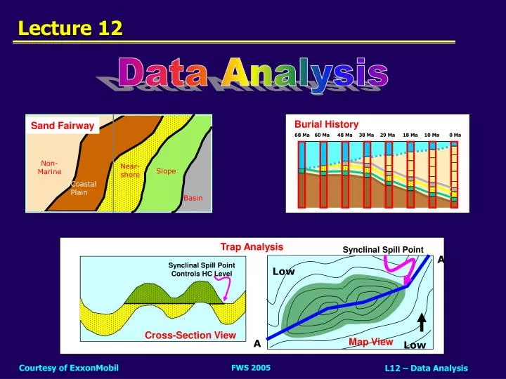
Burial History. Sand Fairway. 68 Ma. 60 Ma. 48 Ma. 38 Ma. 29 Ma. 18 Ma. 10 Ma. 0 Ma. Non- Marine. Near- shore. Slope. Coastal Plain. Basin. Lecture 12. Data Analysis. Trap Analysis. Synclinal Spill Point. A ’. Synclinal Spill Point Controls HC Level. Low.

E N D
Burial History Sand Fairway 68 Ma 60 Ma 48 Ma 38 Ma 29 Ma 18 Ma 10 Ma 0 Ma Non- Marine Near- shore Slope Coastal Plain Basin Lecture 12 Data Analysis Trap Analysis Synclinal Spill Point A’ Synclinal Spill Point Controls HC Level Low Cross-Section View Map View A Low Courtesy of ExxonMobil
Objectives & Relevance • Objective: • Introduce some types of analyses that are used to mature a lead into a prospect once the geologic framework is established • Relevance: Demonstrate some of the scientific methods we use to determine where to drill Courtesy of ExxonMobil
Overview of Data Analysis Once the geologic framework is complete, we can: • Analyze present-day conditions • Where are potential traps? • How much might the trap hold (volume)? • What are the key uncertainties & risks? • Look for geophysical support • DHI and AVO analysis • Model basin fill • When/where have HCs been generated? • How have rock properties changed with time? Courtesy of ExxonMobil
Outline • Time-to-Depth Conversion • Identify Sand Fairways • Identify Traps • Geophysical Evidence • Direct HC Indicators (DHIs) • Amplitude versus Offset (AVO) • Basin Modeling • Back-strip stratigraphy (geohistory) • Forward model (simulation) Courtesy of ExxonMobil
1. Time-to-Depth Conversion Horizons & Faults in units of 2-way time (milliseconds) Velocity Data derived from seismic processing Well Data calibration Time-to-Depth Conversion Horizons & Faults in units of depth (meters or feet) Courtesy of ExxonMobil
Outline • Time-to-Depth Conversion • Identify Sand Fairways • Identify Traps • Geophysical Evidence • Direct HC Indicators (DHIs) • Amplitude versus Offset (AVO) • Basin Modeling • Back-strip stratigraphy (geohistory) • Forward model (simulation) Courtesy of ExxonMobil
2. Identify Sand Fairways For key seismic sequences, namely potential reservoir intervals Reflection Geometries ABC codes Interval Attributes Well Data calibration Seismic Attribute Maps EODs environments of deposition Sand Fairways Courtesy of ExxonMobil
Non- Marine Coastal Plain 10 10 20 30 40 50 20 Near- shore Slope 30 10 20 30 40 50 Basin 40 Example: Nearshore Sands Coastal Plain Nearshore Slope Basin Courtesy of ExxonMobil
Outline • Time-to-Depth Conversion • Identify Sand Fairways • Identify Traps • Geophysical Evidence • Direct HC Indicators (DHIs) • Amplitude versus Offset (AVO) • Basin Modeling • Back-strip stratigraphy (geohistory) • Forward model (simulation) Courtesy of ExxonMobil
3. Identify Traps Use depth (or time) structure maps, with fault zones, to look for places where significant accumulations of HC might be trapped: • Structural traps • e.g., anticlines, high-side fault blocks, low-side roll-overs • Stratigraphic traps • e.g., sub-unconformity traps, sand pinch-outs • Combination traps (structure + stratigraphy) • e.g., deep-water channel crossing an anticline Courtesy of ExxonMobil
Synclinal Spill Point Controls HC Level Structural Traps – A Simple Anticline Synclinal Spill Point If HC charge is great A’ Low A A’ A Low • HCs migrate to anticline • Traps progressively fills down • When HCs reaching the trap is greater, the trap is filled to a leak point • Here there is a synclinal leak point on the east side of the trap Courtesy of ExxonMobil
Structural Traps – A Simple Anticline Synclinal Spill Point If HC charge is limited A’ Low A A’ HC Migrating to Trap Controls HC Level Only enough oil has reached the trap to fill it to this level A Low • HCs migrate to anticline • Traps progressively fills down • When HCs reaching the trap is small, the trap is under-filled – it could hold more • Here the trap is ‘charge-limited’ and is not filled to the synclinal leak point Courtesy of ExxonMobil
A A A’ A’ Synclinal Leak Point Controls HC Level Structural Traps – A Roll-Over Anticline Faulted Anticline – Fault Leaks Faulted Anticline – Fault Seals A A’ A A’ Leak at Fault Controls HC Level Leak Point Leak Point Courtesy of ExxonMobil
Stratigraphic Traps – Sub-Unconformity & Reef A A’ B B’ Upper Sand Lower Sand Upper Sand A A’ B B’ Lower Sand Courtesy of ExxonMobil
Structure + Stratigraphy Cross Section A A A’ Water OIL Water A’ Combo Traps – Channel over an Anticline Structure Stratigraphy A A Low Shale Channel Margin High Channel Axis Channel Margin Shale Low A’ A’ Courtesy of ExxonMobil
Outline • Time-to-Depth Conversion • Identify Sand Fairways • Identify Traps • Geophysical Evidence • Direct HC Indicators (DHIs) • Amplitude versus Offset (AVO) • Basin Modeling • Back-strip stratigraphy (geohistory) • Forward model (simulation) Courtesy of ExxonMobil
What Are DHIs? DHI = Direct Hydrocarbon Indicator • Seismic DHI’s are anomalous seismic responses related to the presence of hydrocarbons • Acoustic impedance of a porous rock decreases as hydrocarbon replaces brine in pore spaces of the rock, causing a seismic anomaly (DHI) • There are a number of DHI signatures; we will look at a few common ones: • Amplitude anomaly • Fluid contact reflection • Fit to structural contours Courtesy of ExxonMobil
Typical Impedance Depth Trends • In general: • Oil sands are lower impedance than water sands and shales • Gas sands are lower impedance than oil sands • The difference in the impedance tends to decrease with depth • The larger the impedance difference between the HC sand and it’s encasing shale, the greater the anomaly IMPEDANCE x 103 5 10 15 20 25 3 4 SHALE OIL SAND Looking for shallow gas 5 6 GAS SAND DEPTH x 103 FEET 7 WATER SAND 8 Looking for deep oil 9 10 Data for Gulf Of Mexico Clastics Courtesy of ExxonMobil
DHIs: Amplitude Anomalies Anomalous amplitudes Change in amplitude along the reflector Low High Amplitude Courtesy of ExxonMobil
DHIs: Fluid Contacts Hydrocarbons are lighter than water and tend to form flat events at the gas/oil contact and the oil/water contact. Thicker Reservoir Fluid contact event Thinner Reservoir Fluid contact event Courtesy of ExxonMobil
DHIs: Fit to Structure Since hydrocarbons are lighter than water, the fluid contacts and associated anomalous seismic events are generally flat in depth and therefore conform to structure, i.e., mimic a contour line Courtesy of ExxonMobil
What is AVO? AVO = Amplitude vs. Offset • We can take seismic data and process it to include all offsets (full stack) or select offsets (partial stacks) • For HC analysis, we often get a near-angle stack and a far-angle stack • The difference in amplitude for a target interval on near vs. far stacks can indicate the type of fluid within the pore space of the rock • AVO analysis examines such amplitude differences Courtesy of ExxonMobil
Some Additional Geophysics Energy Source Receiver Seismic reflections are generated at acoustic boundaries θ θ Layer N Layer N +1 • The amplitude of a seismic reflection • is a function of: • velocities above & below an interface • densities above & below an interface • θ - the angle of incidence of the seismic energy } Change in Impedance Courtesy of ExxonMobil
Why Do We Care? • Reflection amplitude varies with θ as a function of the physical properties above and below the interface • Rock / lithologic properties • Properties of the fluids in the pores • Examining variations in amplitude with angle (or offset) may help us unravel lithology and fluid effects, especially at the top of a reservoir Top of Reservoir Base of Reservoir Impedance Lo Hi Zero Offset Near Offset Full Offset Far Offset Courtesy of ExxonMobil
CDP Gather: HC Leg Time Angle/Offset Water For some reservoirs, the AVO response differs when gas, oil and water fill the pore space Oil AVO: Quantified with 2 Parameters • We quantify the AVO response in terms of two parameters: • Intercept (A) - where the curve intersects 0º • Slope (B) - a linear fit to the AVO data AVO Curve AVO Crossplot • Negative Intercept • Negative Slope Amplitude Angle/Offset AVO Gradient (B) Gas AVO Intercept (A) Courtesy of ExxonMobil
Seismic Example Alpha Fluid Contact? Gas over Oil? Fluid Contact? Oil over Water? Courtesy of ExxonMobil
Analyzing Present-Day Conditions • From present-day configurations, we can: • Predict where Sand Fairways & Source Intervals • Predict EODs and infer lithologies • Evaluate the Trap Configuration • Identify and Size Potential Traps • Consider spill / leak points • Consider if a Sealing Unit Exists • Can shales provide top & lateral seal? • Identify where a distinct HC response occurs • DHI and AVO analysis • Model a simple HC Migration Case • Use present-day dips on stratal units • Assume buoyancy-driven migration Courtesy of ExxonMobil
We Would Like to Know More • We need to incorporate the element of time: • When did the traps form? • When did the source rocks generate HCs? • What was the attitude (dip) of the strata when the HCs were migrating? • What is the quality of the reservoir (Φ , k) • How adequate is the seal? • How have temperature and pressure conditions changed through time? To answer these questions, we have to model the basin’s history from the time of deposition to the present Courtesy of ExxonMobil
Outline • Time-to-Depth Conversion • Identify Sand Fairways • Identify Traps • Geophysical Evidence • Direct HC Indicators (DHIs) • Amplitude versus Offset (AVO) • Basin Modeling • Back-strip stratigraphy (geohistory) • Forward model (simulation) Courtesy of ExxonMobil
Back-strip the Present-day Strata to Unravel the Basin’s History Model Rock & Fluid Properties Forward through Time 18 Ma Time Steps are Limited to Mapped Horizons Time Steps are Regular Intervals as Defined by the User 29 Ma 36 Ma 42 Ma Basin Modeling 0 Ma Courtesy of ExxonMobil
Basin Modeling • We start with the present-day stratigraphy • Then we back-strip the interpreted sequences to get information of basin formation and fill • For some basins, we can deduce a heat flow history from the subsidence history (exercise) • Next we model basin fill forward through time at a uniform time step (typically ½ or 1 Ma) • If we have well data, we check our model • Temperature data • Organic maturity (vitrinite reflectance) • Porosity • Given a calibrated basin model, we predict • HC generation from source intervals • Reservoir porosity Courtesy of ExxonMobil
Spillage of Excess Gas Migration Path Of Spilled Oil “Gas separator” Simple Model of HC Migration • Generate oil and gas at lower left • HCs ‘percolate’ into porous interval (white) • Trap A fills with oil and gas – gas displaces oil • Trap B fills with spilled oil and gas • Seal at B will only hold a certain thickness of gas • At trap B – gas leaks while oil spills Trap C Trap B Trap A Traps with unlimited charge Source Generating HCs Courtesy of ExxonMobil
A1 Gas Sand Figure 1 Inline 840 Intro to Exercise Goal: To map the extent of the A1 gas-filled reservoir W E Courtesy of ExxonMobil
Inline 840 Changes in Amplitude Indicate Fluid Gas Sand Water Sand Traces are ‘clipped’ Figure 1 Courtesy of ExxonMobil
Inline 840 Figure 1 Fluids within the A1 Sand Extent of Gas Courtesy of ExxonMobil