Download
1 / 57
570 likes | 697 Views
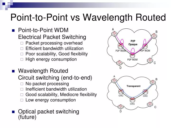
Point-to-Point WDM Electrical Packet Switching Packet processing overhead Efficient bandwidth utilization Poor scalability, Good flexibility High energy consumption Wavelength Routed Circuit switching (end-to-end) No packet processing Inefficient bandwidth utilization

E N D
Point-to-Point WDM Electrical Packet Switching Packet processing overhead Efficient bandwidth utilization Poor scalability, Good flexibility High energy consumption Wavelength Routed Circuit switching (end-to-end) No packet processing Inefficient bandwidth utilization Good scalability, Mediocre flexibility Low energy consumption Optical packet switching (future) Point-to-Point vs Wavelength Routed
OXC Architecture Optical Cross Connect (OXC)
Μετατροπέας μηκών κύματος (wavelength converter): λειτουργικότητα και χαρακτηριστικά • Ένας ιδανικός μετατροπέας μηκών κύματος έχει τα ακόλουθα χαρακτηριστικά: • - διαφάνεια στους ρυθμούς bit και στις διαμορφώσεις σημάτων • ταχύς χρόνος προετοιμασίας του μήκους κύματος εξόδου • μετατροπή τόσο στα κοντύτερα όσο και στα μακρύτερα μήκη κύματος • δυνατότητα για ίδια μήκη κύματος εισόδου και εξόδου (όχι μετατροπή) • αναισθησία στην πόλωση των σημάτων εισόδου • low-chirp σήμα εξόδου με υψηλό λόγο ‘απόσβεσης’ και πολύ μεγάλο λόγο • σήματος-προς-θόρυβο • απλή υλοποίηση
Αραιή μετατροπή μηκών κύματος • αραιή κομβική μετατροπή: δίνει μόνο σε ένα περιορισμένο αριθμό κόμβων • πλήρεις δυνατότητες μετατροπής • αραιή μετατροπή εξόδων μεταγωγέων: χρησιμοποιεί μεταγωγείς που • μοιράζονται ένα περιορισμένο πλήθος μετατροπέων μηκών κύματος • αραιή (ή περιορισμένη) μετατροπή εύρους: δίνει μόνο ένα περιορισμένο • εύρος στους μεταγωγείς που αναπτύσσονται, εξαιτίας περιορισμένου κόστους • και ισχύος Αραιή μετατροπή εύρους εύρος μετατροπής = 1
Διαφανές οπτικό δίκτυο Αδιαφανές οπτικό δίκτυο εγκαθιστά end-to-end μονοπάτια φωτός κατά μήκος του δικτύου αναπαράγει τα σήματα σε κάθε hop στο δίκτυο Ημιδιαφανές οπτικό δίκτυο • αναπαράγει τα σήματα μόνο όταν είναι απαραίτητο • ιδέα των σταθμών ανεφοδιασμού • αναπαραγωγή στον κόμβο στα μισά του δρομολογίου
Routing and Wavelength Assignment problem (RWA) (without wavelength conversion at the nodes)
Μοντελοποίηση του μήκους των μονοπατιών λογισμικό ελέγχου • ανάθεση κόστους σε κάθε μετατροπέα μηκών κύματος • κόστος ενός μονοπατιού για μια σύνδεση = κόστος συνδέσμων + • κόστος μετατροπής μηκών κύματος • το μονοπάτι μικρότερου κόστους περιλαμβάνει κόστη συνδέσμων • και κόστη μετατροπών μηκών κύματος
Μονοπάτια φωτός και δρομολόγηση μηκών κύματος • μονοπάτι φωτός • εικονική τοπολογία • περιορισμός συνέχειας μηκών • κύματος • μετατροπή μηκών κύματος • δρομολόγηση • φραγμένο μήκος μονοπατιών • φωτός Εικονική τοπολογία
Protection Mechanisms The 1+1 protection. No protocol is needed Working fibre Protection fibre The 1:1 and 1:N protection. Signaling protocol is needed 1+1 is faster than 1:1 but in the latter case the spare fibre could be used for low priority traffic (extra Tx, Rx)
What should be protected? Path protection Note that rerouting is handled by source-destination nodes. Link protection: In (a) the traffic is re-routed to a different fibre in (b) each channel may take a different route. b a
Wavelength Routing Pros and Cons • Setting up a lightpath is like setting up a circuit (a 2-way process with Req and Ack): RTT = tens of ms • Pros: • good for smooth traffic • Mature OXC technology (msec switching time) • QoS guarantee due to fixed BW reservation • Cons: BW inefficient for bursty (data) traffic • wasted BW during off/low-traffic periods • very coarse granularity (OC-48 and above) • limited # of wavelengths (thus # of lightpaths)
Wavelength-Routed WDM networks • Physical topology: A set of routing nodes connected by fiber links • Optical Cross-connect - OXC: No O-E-O conversion • Lightpath: A lightpath has to be setup before the data transmission. A Lightpath remains in the optical domain from src to dst • Logical topology: The set of src-dst pairs connected through lightpaths OXC OXC Wavelength reuse # wavelengths << # OXCs OXC OXC OXC OXC OXC Routing and Wavelength Assignment
RWA: Routing and Wavelength Assignment • Definition • Given: network topology, end-to-end connection requests • Problem: Determine routes and wavelengths for the requests • Offline RWA (network planning phase) • The entire set of requests are given in advance (traffic matrix). • Online RWA (network operation phase) • Requests arrive randomly over time and are served one-by-one • Objective: Minimizing the Overall Blocking Probability
Transparent wavelength routed networks • All-optical transparent networks: advantages in capacity, cost and energy • The transmission quality is affected by physical layer impairments (PLIs) • Physical layer blocking: the signal detection at the receiver may be infeasible • Impairment aware (IA)-RWA algorithms
Pure RWA - problem definition • Input: • Network topology: connected graph G=(V,E) • V: set of nodes, assumed not to be equipped with wavelength converters • E: set of point-to-point single-fiber links • Each fiber is able to support a set C={1,2,…,W} of W distinct wavelengths • A-priori known traffic scenario given in a matrix of nonnegative integers Λ • Output: • the RWA instance solution, in the form of routes and assigned wavelengths • the number of wavelengths required to route all the connections • Objective: minimize the number of used wavelengths
cost3x1 + 2x2 IntegerLinear Programming(ILP) • Integer variablesx minimize cT.x subject to A.x ≤ b, x = (x1,...,xn) ∈ Ζn • The general ILP problem is NP-complete • Algorithms • Solve small-medium size ILP problems • Branch-and-bound • Cutting plane • Mixed Integer Linear Programming (MILP): integer and float variables ONDM 2011, Bologna, Italy
Convex Hall • The same set of integer solutions can be described by different sets of constraints (the same set of integer solutions can be included in different-shaped n-dimensional polyhedrons) • The convex hull is the minimum convex set that includes all the integer solutions of the problem • Given the convex hull we can use a LP algorithm to obtain the optimal ILP solution in polynomial time • The transformation of a general n-dimension polyhedron to the corresponding convex hull is difficult (process used in cutting plane techniques) • Good ILP formulation: the feasible region defined by the linear constraints is close (tight) to the corresponding convex hull • A large number of vertices consist of integer variables. This increases the probability of obtaining an integer solution when solving the corresponding LP-relaxation of the initial ILP problem ONDM 2011, Bologna, Italy
LP Formulation and Flow Cost Function Flow Cost Function • Increasing and Convex (to imply a greater amount of ‘undesirability’ when a link becomes congested) • Approximated by a piecewise linear function • Integer break points (makes Simplex yield integer optimal solutions with high probability) We obtain integer solutions in 98% of the problem instances!
Random perturbation • In the general multicommodity problem, a flow that is served by more than one paths has equal sum of first derivates over the links of those paths • In our problem a request that is served by more than one lightpaths has equal sums of first derivates over the links of these paths • To avoid such cases, we multiply the slopes of each variable on each link with a random number that is close to 1 • In this way, the cases that two variables have equal derivates over the links that comprise a path are reduced, and thus we obtain more integer solutions
Handling non-integer solutions • Make Simplex yield integer optimal solutions • Piecewise linear cost functions • Random perturbation technique • Still the solution may be non-integer • Iterative fixings • Fix the integer variables of the solutions and solve the remaining (reduced) LP problem • The objective cost does not change if we get to an integer solution it is optimal • When fixing does not further increase the integrality, we proceed to the rounding process • Iterative rounding • Round a single variable, the one closest to 1, and continue solving the reduced LP problem • Rounding helps us move to a higher objective and search for an integer solution there • If the objective changes we are not sure anymore that we will find an optimal solution
Pure RWA algorithm Use a pure RWA algorithm that is based on a LP-relaxation formulation The algorithm consists of 4 steps 1. We calculate a set of candidate paths 2. Using the set of candidate paths we formulate the RWA instance as a LP problem and use Simplex to solve it 3. We handle a fractional (non-integer) solution, by applying iterative fixing and rounding methods 4. We handle non infeasible instances (when the RWA instance cannot be served with the given number of wavelengths)
IA-RWA problem • IA-RWA objective: minimize the number of wavelengths used (network layer) and also select lightpaths with acceptable transmission quality (physical layer) • For IA-RWA algorithms we classify physical layer impairments (PLIs) into: • 1st class PLIs: generated by the same lightpath (ASE, CD, PMD, FC, SPM) • 2nd class PLIs: generated due to inter-lightpath interference (XT, XPM, FWM) • PLIs of the 2nd class make routing decisions for one lightpath affect and be affected by decisions made for the other lightpaths • Solution: • Worst case interference assumption • Actual interference: cross layer optimization
Worst Case and Actual Interference Actual interference: cross layer optimization algo: • Consider PLIs that do not depend on interference (1st class PLIs) • Prune candidate lightpaths that do not have acceptable QoT • Formulate the interference among lightpaths into the RWA Worst case interference algo: • Consider PLIs that do not depend on interference (1st class PLIs) • Assume all wavelengths active (2nd class PLIs) • Prune candidate lightpaths that do not have acceptable QoT Illustrative example: DTnet topology - single connection request between all (s,d) pairs The reduction in the solution space can deteriorate wavelength performance
Physical layer evaluation: Q-factor • Use the Q factor to estimate the feasibility of a lightpath • The Q factor is related to the BER • Analytical formulas can be used to calculate the Q factor
Proposed IA-RWA algorithms • Indirect IA-RWA algo: Constrain the impairment generating sources • the length and the number of hops of a path • the number of adjacent (and second adjacent) channels over all links of the lightpath • the number of intra-channel generating sources (lightpaths crossing the same switch utilizing the same wavelength) along the lightpath • Direct IA-RWA algo: Use the definition of Q factor and noise variance related parameters to define physical layer constraints into the RWA
Indirect (Parametric) IA-RWA algo Number of active adjacent channels (Affected PLIs: Intra-XT, XPM and FWM) Number of intra-channel XT sources (Soft) constrain the number of adjacent channel interfering sources on lightpath (p,w) B is a large constant used to activate/deactivate the constraint Similarly we constrain the second-adjacent channel interfering sources (Soft) constrain the number of intra-XT interfering sources on lightpath (p,w) B is a large constant used to activate/deactivate the constraint Similarly we constrain the second-adjacent channel interfering sources Carry the surplus variables in the minimization objective
Direct (Sigma Bound) IA-RWA algo • For each candidate lightpath (p,w) inserted in the RWA formulation, we calculate an upper bound on the interference noise variance it can tolerate, after accounting for the impairments that do not depend on the utilization of the other lightpaths (account for 1st Class PLIs). • Then using noise-variance related parameters per link we can constrain the interference (due to 2nd Class PLIs) accumulated on lightpath (p,w) • If the selected lightpaths satisfy these constraints they have, by definition, acceptable quality of transmission
Performance evaluation results • Simulation platform Matlab + LINDO API • Generic DT network topology • Traffic Scenarios • Random traffic matrix generator • DTnet actual traffic matrix • Physical Layer Evaluation: Q-Tool • Uses analytical models to calculate the Q factor of lightpaths • Realistic physical layer parameters
Pure RWA performance • 100 RWA instances • ILP min-max: optimality criterion • LP min-max: running time & integrality criteria • The proposed LP-relaxation+piecewise linear costs has superior performance • The performance is Improved with the random perturbation technique
Indirect and Direct IA-RWA • 100 RWA instances • W=16 available wavelengths • Algorithms: • Pure RWA • Indirect P-IA-RWA • Direct SB-IA-RWA • The proposed IA-RWA algorithms reduce the (physical layer) blocking • Additional wavelengths are required to spread the lightpaths and avoid interference • The direct SB-IA-RWA algo can find zero blocking solutions • The direct SB-IA-RWA algo maintains zero blocking up to ρ=0.8, after which the 16 available wavelengths are not enough
Direct IA-RWA algo performance • Direct SB-IA-RWA algorithm, solved using • The proposed LP-relaxation technique • ILP • 100 random RWA instances • Find zero blocking solutions • Using ILP we were able to solve all instances within 5 hours up to ρ=0.7 load • Using the LP-relaxation the optimality is lost in 2 or 3 instances but the execution time is maintained very low
Realistic traffic matrix • Realistic traffic matrix (381 connections load ρ=2.05) • The propose IA-RWA algorithms reduce the physical layer blocking • The direct SB-IA-RWA finds zero blocking solution • with W=36 • Running time: 20 minutes acceptable for the realistic network and traffic load
Dynamic ΙΑ-RWA Algorithm • Input: New connection request Current network state • Objective: serve the connections and minimize blocking over (infinite) time • We use a multicost algorithm with 2 phases • Calculate the set of non-dominated paths from the given source to the given destination • Choose the lightpath that minimizes the objective function
Calculating the Set of Non-Dominated Paths • Cost vector of link l: Vector maps the utilization of wavelengths • The cost vector of path pcan be calculated based on the cost vectors of links l=1,2,...,m, that comprise it • The cost parameters of a path can be combined so as to calculate the Q factors of the available lightpaths over that path • Prune the solution space • For each p, we check the Q factor of available lightpaths and we make unavailable those that do not have acceptable performance • Σταματάμε να επεκτείνουμε μονοπάτια αν δεν έχουν τουλάχιστον ένα διαθέσιμο μήκος κύματος
Qmax Q Q Qmax Q dmin dmin Calculating the Set of Non-Dominated Paths Domination relationship between two paths p1 dominates p2 (p1 > p2) iff • Using the above definitions we use a multicost algorithm, which is a generalization of Dijkstra algorithm, to compute the set of non-dominated paths Pn-d from the given source to the given destination • By definition, the paths that are included in Pn-dhave • At least one available wavelength • The available wavelength have acceptable transmission performance (Q factor)
Optimization Policies We evaluated 3 optimization policies (that correspond to 3 different IA-RWA algorithms) i) Most Used Wavelength (MUW) We order the lightpaths to decreasing wavelength utilization order and select the one that is used more in the network. ii) Better Q performance (bQ) We select the lightpath with the higher Qfactor value iii) Mixed better Q and most used wavelength (bQ-MUW) From the set of available lightpaths we select those with Q values no less than 0.5dB than the highest Q value and then apply the MUW policy to this new set of lightpaths
Mixed Line Rates WDM Networks • Several Line Rates (10/40/100)Gbps • Exploit the MLR heterogeneity to reduce the cost of the network • Long-distance low-bit-rate connections could be served with inexpensive low-rate and long-reach (e.g. 10 Gbps) transponders • High bit-rate connections could be served with more expensive higher-rate transponders. Typically, higher rate transponders have shorter reach • Interference among lightpaths of different rates • Mixed Line Rates RWA algorithms
Transmission Reach & Effective Length • Rates: r={10,40,100}Gbps • Fiber types: t={{10}, {40}, {100}, {10,40}, {10,100}, {40,100}, {10,40,100}} • Interference between different modulation format/rates • mr,t≥1: the increase of the length of the link for a connection of rate r, due to interference effects generated by the other modulation formats/rates concurrently transmitted over the fiber t • mr,t≡{r}=1: a fiber (t≡{r}) is used only by connections of a certain rate r(its effective length is equal to its real length) • Length of link l: • Maximum transmission reach at r : • Effective length of fiber t for a transmission of rate r • Effective length of the path p at rate r • Satisfy:
Transmission Reach & Effective Length • AC and CB are t={10} • AB is t={10,40} • Effective length of the path pACB at rate 10 • Effective length of the path pABD at rate 10 • m10,{10}=1 • m10,{10,40} ≥ 1 • Length of link l: • Maximum transmission reach at r : • Effective length of fiber t for a transmission of rate r • Effective length of the path p at rate r • Satisfy:
MLR RWA - Problem Definition • Input: • Network topology: graph G=(V,E) V: set of nodes (no wavelength conversion), E: set of point-to-point single-fibers • Each fiber supports C={1,2,…,W}: W distinct wavelengths, R={r1,r2,…,rM}: M different bit rates • A-priori known traffic scenario given in a matrix Λ of requested bandwidth • Output: The RWA instance solution, in the form of routes, assigned wavelengths and bit rates • Objective: minimize the network cost related to the number and the type of the transponders used • Constraints: single wavelength assignment, wavelength continuity, transmission reach (based on effective length)
ILP Formulation Cost of the transponder at rate r Minimize the total cost of the transponders
ILP Formulation Enable/disable the use of a certain path for a certain rate based on the effective lengths of the links that it comprise it utilization of different rates of a link type of fiber used on link Prohibit the utilization of lightpaths over paths that cannot be used for a transmission at a certain rate ONDM, Bologna, 2011
Performance Evaluation Results • Simulation platform: Matlab + CPLEX • Generic DT network topology • 14 nodes • 46 directed links • Traffic Scenarios • DTnet actual traffic matrix • range from 4.5 up to 47 Gbps • average 15 Gbps • Scale up to 8 times • Fiber types • T={{10},{40},{10,40}} • Costs and maximum reach • C10=1, D10=2500 km, C40=2.5, D40=800 km
Performance Evaluation Results Heuristics For comparison purposes Lower bound of network cost: No interference between different rates For comparison purposes Network planning under worst case interference assumption Da40=800/1.25=640 km Multiplier factor Number of fiber types used per load Even at high loads the ILP algorithm manages to have a high number of links that support only 40 Gbps connections